Electromagnetic Fields PYQ Set (2000 to 2025)
Solution =
⦾ Faraday’s Law and Curl of Electric Field
In a region where both electric and magnetic fields are time-invariant, Faraday’s Law ensures that:
⦾ Step 1:
Faraday’s Law of Induction is given by: \[ \nabla \times \mathbf{E} = – \frac{\partial \mathbf{B}}{\partial t} \] where: – \( \mathbf{E} \) is the electric field, – \( \mathbf{B} \) is the magnetic field, – \( \frac{\partial \mathbf{B}}{\partial t} \) represents the time rate of change of the magnetic field.
⦾ Step 2:
When both the electric and magnetic fields are time-invariant (i.e., no time-varying magnetic field), the term \( \frac{\partial \mathbf{B}}{\partial t} \) becomes zero. \[ \nabla \times \mathbf{E} = 0 \] This means the curl of the electric field is zero, indicating that the electric field is conservative and can be derived from a potential function.
⦾ Step 3:
Therefore, the correct Maxwell equation that ensures \( \nabla \times \mathbf{E} = 0 \) in this case is Faraday’s Law.
⦾ Answer: The Maxwell equation that ensures \( \nabla \times \mathbf{E} = 0 \) when both fields are time-invariant is Faraday’s Law
Solution =
To determine the input impedance of a short-circuited lossless transmission line of length less than a quarter wavelength, we need to analyze the behavior of such a transmission line.
⦾ Key Concepts:
Short-Circuited Transmission Line: When a transmission line is short-circuited, the load impedance \( Z_L \) is zero.
Input Impedance: The input impedance \( Z_{in} \) of a transmission line of length \( l \) and characteristic impedance \( Z_0 \) is given by: \[ Z_{in} = Z_0 \frac{Z_L + j Z_0 \tan(\beta l)}{Z_0 + j Z_L \tan(\beta l)} \] where \( \beta = \frac{2\pi}{\lambda} \) is the phase constant, and \( \lambda \) is the wavelength.
Short-Circuit Condition: For a short-circuited line (\( Z_L = 0 \)): \[ Z_{in} = j Z_0 \tan(\beta l) \]
⦾ Analysis:
For a lossless transmission line, \( Z_0 \) is purely real.
The term \( \tan(\beta l) \) depends on the length \( l \) of the line relative to the wavelength \( \lambda \).
⦾ Length Less Than a Quarter Wavelength:
If \( l < \frac{\lambda}{4} \), then \( \beta l < \frac{\pi}{2} \).
In this range, \( \tan(\beta l) \) is positive.
Therefore, \( Z_{in} = j Z_0 \tan(\beta l) \) is purely imaginary and positive, indicating a purely inductive reactance.
⦾ Final Answer: b) purely inductive
Solution =
The given electric field is:
\[ \mathbf{E} = \bigl(a_x + j 4 a_y\bigr) e^{j(2\pi \times 10^7 t – 0.2z)} \]
⦾ Step 1: Extract Components
Let:
\[ E_x = a_x, \quad E_y = 4j. \]
Since \( E_y \) has a factor of \( j = e^{j\pi/2} \), it has a phase lead of \( +90^\circ \) over \( E_x \).
⦾ Step 2: Convert to Time Domain
Taking the real part, define \( \phi = 2\pi \times 10^7 t – 0.2z \), then:
\[ E_x(t) = \cos(\phi) \]
\[ E_y(t) = -4 \sin(\phi). \]
At \( (t,z) = (0,0) \):
\[ E_x(0) = 1, \quad E_y(0) = 0. \]
⦾ Step 3: Determine Rotation Direction
For \( \phi = \pi/2 \):
\[ E_x(\pi/2) = 0, \quad E_y(\pi/2) = -4. \]
The vector moves from \( (+x, 0) \) to \( (0, -4) \), indicating **clockwise** rotation when viewed along the direction of wave propagation \( +z \).
Clockwise rotation means the wave is **right-handed**.
⦾ Step 4: Check for Circular vs Elliptical
Since the amplitudes are different (\(1\) for \( E_x \), \(4\) for \( E_y \)), the trajectory is an **ellipse**, not a perfect circle.
⦾ Final Answer: (b) Right-Handed Elliptical Polarization
Solution =
Electromagnetic Wave Propagation in Free Space For a propagating electromagnetic wave in free space, the relationship between the electric field \( \mathbf{E} \), magnetic field \( \mathbf{B} \), and the direction of wave propagation \( \mathbf{k} \) is crucial. These vectors are always mutually perpendicular in a uniform wave propagation.
⦾ Step 1: In a propagating electromagnetic wave, the electric field \( \mathbf{E} \), magnetic field \( \mathbf{B} \), and the wave vector \( \mathbf{k} \) (which indicates the direction of propagation) satisfy the following condition: \[ \mathbf{E} \perp \mathbf{B} \perp \mathbf{k} \] This means: – The electric field \( \mathbf{E} \) is perpendicular to the magnetic field \( \mathbf{B} \), – The magnetic field \( \mathbf{B} \) is perpendicular to the direction of propagation \( \mathbf{k} \), – The electric field \( \mathbf{E} \) is also perpendicular to the direction of propagation \( \mathbf{k} \).
⦾ Step 2: This relationship holds true for all electromagnetic waves traveling through free space.
⦾ Step 3: Therefore, the correct statement about the relationship between \( \mathbf{E} \), \( \mathbf{B} \), and \( \mathbf{k} \) is: \[ \mathbf{E} \perp \mathbf{B} \perp \mathbf{k} \]
⦾ Answer: The correct relationship for the electric field, magnetic field, and wave propagation direction is \[ \mathbf{E} \perp \mathbf{B} \perp \mathbf{k} \]
Solution =
Maxwell’s equations describe the fundamental behavior of electromagnetic fields. One of these equations represents the absence of magnetic monopoles.
⦾ Step 1: The equation that describes the absence of magnetic monopoles is: \[ \nabla \cdot \mathbf{B} = 0 \] This equation tells us that the magnetic field \( \mathbf{B} \) has no divergence, meaning there are no isolated magnetic charges, or magnetic monopoles.
⦾ Step 2: In other words, magnetic field lines are always closed loops, and there are no “north” or “south” magnetic charges like there are for electric fields.
⦾ Step 3: This is in contrast to electric field lines, which can originate from positive charges and terminate at negative charges. Magnetic field lines, however, must always form loops or extend to infinity.
⦾ Answer: The equation that represents the absence of magnetic monopoles is \( \nabla \cdot \mathbf{B} = 0 \)
Solution =
The skin depth \( \delta \) in a conductor can be calculated using the following formula:
⦾ Step 1: The skin depth formula is: \[ \delta = \sqrt{\frac{2}{\mu \sigma \omega}} \] Where: – \( \mu \) is the permeability of the material (for free space, \( \mu_0 = 4\pi \times 10^{-7} \, \text{H/m} \)), – \( \sigma \) is the conductivity of the material (given as \( 5.8 \times 10^7 \, \text{S/m} \)), – \( \omega \) is the angular frequency, given by \( \omega = 2 \pi f \), where \( f \) is the frequency of the wave (given as \( 1 \, \text{MHz} = 10^6 \, \text{Hz} \)).
⦾ Step 2:
First, calculate the angular frequency \( \omega \): \[ \omega = 2 \pi f \] \[ \omega = 2 \pi \times 1 \times 10^6 \, \text{Hz} = 6.2 \times 10^6 \, \text{rad/s} \]
⦾ Step 3: Now, substitute the values into the skin depth formula: \[ \delta = \sqrt{\frac{2}{\mu_0 \sigma \omega}} \] \[\frac{2}{(4\pi \times 10^{-7}) \times (5.8 \times 10^7) \times (6.2 \times 10^6)} \]
⦾ Simplify the expression: \[\frac{2}{(1.2 \times 10^{-6}) \times (5.8 \times 10^7) \times (6.2 \times 10^6)} \] \[ \delta = \sqrt{\frac{2}{(4.315 \times 10^8)}} \] \[ \delta = \sqrt{4.634 \times 10^{-9}} \] \[ \delta = 6.80 \times 10^{-5} \, \text{mm} = 68 \, \mu\text{m} \]
The skin depth \( \delta \) is 68 μm.
⦾ Answer: The closest value is (B) 68 μm.
Solution =
⦾ Velocity of Electromagnetic Waves in a Material
Given a material with permittivity \( \epsilon = 2 \epsilon_0 \) and permeability \( \mu = 3 \mu_0 \), we will calculate the velocity of electromagnetic waves in the material.
⦾ Step 1:
The velocity of electromagnetic waves in a material is given by: \[ v = \frac{1}{\sqrt{\mu \epsilon}} \] where \( v \) is the velocity, \( \mu \) is the permeability, and \( \epsilon \) is the permittivity.
⦾ Step 2:
Substitute the given values \( \epsilon = 2 \epsilon_0 \) and \( \mu = 3 \mu_0 \) into the formula: \[ v = \frac{1}{\sqrt{(3 \mu_0)(2 \epsilon_0)}} \]
⦾ Step 3:
Simplify the equation: \[ v = \frac{1}{\sqrt{6 \mu_0 \epsilon_0}} \] Since \( \frac{1}{\sqrt{\mu_0 \epsilon_0}} = c \) (the speed of light in a vacuum), we have: \[ v = \frac{c}{\sqrt{6}} \]
⦾ Answer: The velocity of electromagnetic waves in this material is (B) \( \frac{c}{\sqrt{6}} \)
Solution =
Magnetic Field at the Surface of a Conductor To calculate the magnetic field \( B \) at the surface of a cylindrical conductor carrying a uniformly distributed current, we use the formula:
\[ B = \frac{\mu_0 I}{2 \pi r} \] Where: – \( \mu_0 = 4\pi \times 10^{-7} \, \text{H/m} \) (permeability of free space), – \( I = 5 \, \text{A} \) (current), – \( r = 1 \, \text{mm} = 1 \times 10^{-3} \, \text{m} \) (radius of the conductor).
⦾ Step 1: Substitute the values into the formula: \[ B = \frac{\mu_0 I}{2 \pi r} \] \[ B = \frac{(4 \pi \times 10^{-7}) \times 5}{2 \pi \times (1 \times 10^{-3})} \]
⦾ Step 2: Simplify the expression: \[ B = \frac{4 \pi \times 5 \times 10^{-7}}{2 \pi \times 10^{-3}} \] \[ B = \frac{20 \pi \times 10^{-7}}{2 \pi \times 10^{-3}} \]
⦾ Step 3: Cancel \( \pi \) and simplify further: \[ B = \frac{20 \times 10^{-7}}{2 \times 10^{-3}} \] \[ B = 10 \times 10^{-4} = 0.001 \, \text{T} \]
⦾ Step 4: Convert to mT: \[ B = 1 \, \text{mT} \]
The magnetic field at the surface of the conductor is 1 mT.
⦾ Answer: The correct option is (A) 1 mT.
Solution =
To calculate the phase velocity \( v_p \) of an electromagnetic wave in a lossless dielectric medium, we use the formula:
\[ v_p = \frac{c}{\sqrt{\epsilon_r \mu_r}} \] ⦾ Where: – \( c = 3 \times 10^8 \, \text{m/s} \) (speed of light in free space), – \( \epsilon_r = 4 \) (relative permittivity of the medium), – \( \mu_r = 1 \) (relative permeability of the medium).
⦾ Step 1: Substitute the given values into the formula: \[ v_p = \frac{3 \times 10^8}{\sqrt{\epsilon_r \mu_r}} \] \[ v_p = \frac{3 \times 10^8}{\sqrt{4 \times 1}} \]
⦾ Step 2: Simplify the denominator: \[ v_p = \frac{3 \times 10^8}{\sqrt{4}} \] \[ v_p = \frac{3 \times 10^8}{2} \]
⦾ Step 3: Perform the division: \[ v_p = 1.5 \times 10^8 \, \text{m/s} \]
The phase velocity in the dielectric medium is \( 1.5 \times 10^8 \, \text{m/s} \).
⦾ Answer: The correct option is (A) \( 1.5 \times 10^8 \, \text{m/s} \).
Solution =
The magnitude of the reflection coefficient \( \Gamma \) for a transmission line is calculated using the formula:
\[ \Gamma = \left| \frac{Z_L – Z_0}{Z_L + Z_0} \right| \] Where: – \( Z_L = 150 \, \Omega \) (load impedance), – \( Z_0 = 75 \, \Omega \) (characteristic impedance).
⦾ Step 1: Substitute the given values: \[ \Gamma = \left| \frac{150 – 75}{150 + 75} \right| \]
⦾ Step 2: Simplify the numerator: \[ \Gamma = \left| \frac{75}{150 + 75} \right| \]
⦾ Step 3: Simplify the denominator: \[ \Gamma = \left| \frac{75}{225} \right| \]
⦾ Step 4: Perform the division: \[ \Gamma = 0.333\ldots \]
⦾ Step 5: Round to two decimal places: \[ \Gamma \approx 0.33 \]
The magnitude of the reflection coefficient is \( 0.33 \).
⦾ Answer: The correct option is (C) 0.33.
Solution =
Given that the capacitor has two dielectrics with relative permittivities \( \epsilon_1 \) and \( \epsilon_2 \), occupying equal thickness, the equivalent capacitance \( C_{\text{eq}} \) can be calculated using the following formula:
⦾ Step 1: The total capacitance for two dielectrics in series is given by:
\[ \frac{1}{C_{\text{eq}}} \] \[ = \frac{1}{C_1} + \frac{1}{C_2} \] Where \( C_1 \) and \( C_2 \) are the capacitances for each dielectric material.
⦾ Step 2: The capacitance for dielectric 1 is given by:
\[ C_1 = \frac{\epsilon_1 \epsilon_0 A}{d/2} \] \[ = \frac{2 \epsilon_1 \epsilon_0 A}{d} \] Where \( \epsilon_1 \) is the relative permittivity of dielectric 1, \( \epsilon_0 \) is the permittivity of free space, \( A \) is the plate area, and \( d \) is the plate separation.
⦾ Step 3: Similarly, the capacitance for dielectric 2 is given by:
\[ C_2 = \frac{\epsilon_2 \epsilon_0 A}{d/2} \] \[ = \frac{2 \epsilon_2 \epsilon_0 A}{d} \] Where \( \epsilon_2 \) is the relative permittivity of dielectric 2.
⦾ Step 4: Substituting \( C_1 \) and \( C_2 \) into the formula for \( C_{\text{eq}} \), we get:
\[ \frac{1}{C_{\text{eq}}} \] \[ = \frac{d}{2 \epsilon_0 A} \left( \frac{1}{\epsilon_1} + \frac{1}{\epsilon_2} \right) \] Now, this gives us the reciprocal of the equivalent capacitance as a function of the two dielectrics’ permittivities.
⦾ Step 5: Solving for \( C_{\text{eq}} \), we get:
\[ C_{\text{eq}} = \frac{2 \epsilon_0 A}{d} \times \frac{\epsilon_1 \epsilon_2}{\epsilon_1 + \epsilon_2} \] So, the equivalent capacitance is given by: \[ C_{\text{eq}} = \frac{2 \epsilon_0 A}{d} \times \frac{\epsilon_1 \epsilon_2}{\epsilon_1 + \epsilon_2} \]
The final formula for the equivalent capacitance is:
\[ C_{\text{eq}} = \frac{2 \epsilon_0 A}{d} \times \frac{\epsilon_1 \epsilon_2}{\epsilon_1 + \epsilon_2} \]
Answer: The correct option is (B).
Solution =
The power density \( S \) of a uniform plane wave in free space is calculated using the formula:
\[ S = \frac{E^2}{2 \eta_0} \] Where: – \( S \) is the power density in \( \text{W/m}^2 \), – \( E = 120 \, \text{V/m} \) (electric field amplitude), – \( \eta_0 = 377 \, \Omega \) (intrinsic impedance of free space).
⦾ Step 1: Substitute the given values into the formula: \[ S = \frac{120^2}{2 \times 377} \]
⦾ Step 2: Calculate the numerator: \[ 120^2 = 14400 \]
⦾ Step 3: Calculate the denominator: \[ 2 \times 377 = 754 \]
⦾ Step 4: Perform the division: \[ S = \frac{14400}{754} \approx 19.1 \, \text{W/m}^2 \]
The power density is 19.1 W/m².
⦾ Answer: The correct option is (C) 19.1.
Solution =
The electric field \( E \) just outside the surface of a charged spherical conductor is calculated using the formula:
\[ E = \frac{Q}{4 \pi \epsilon_0 r^2} \] Where: – \( Q = 2 \, \mu C = 2 \times 10^{-6} \, C \) (charge on the sphere), – \( r = 10 \, \text{cm} = 0.1 \, \text{m} \) (radius of the sphere), – \( \epsilon_0 = 8.854 \times 10^{-12} \, \text{F/m} \) (permittivity of free space).
⦾ Step 1: Substitute the values into the formula: \[ E = \frac{2 \times 10^{-6}}{4 \pi (8.854 \times 10^{-12}) (0.1)^2} \]
⦾ Step 2: Calculate \( (0.1)^2 \): \[ (0.1)^2 = 0.01 \]
⦾ Step 3: Multiply \( 4 \pi \epsilon_0 \): \[ 4 \pi \epsilon_0 = 4 \pi \times 8.85 \times 10^{-12} \approx 1.11 \times 10^{-10} \]
⦾ Step 4: Calculate the denominator: \[ (1.112 \times 10^{-10}) \times 0.01 = 1.112 \times 10^{-12} \]
⦾ Step 5: Divide \( Q \) by the denominator: \[ E = \frac{2 \times 10^{-6}}{1.112 \times 10^{-12}} \approx 1.8 \times 10^{6} \, \text{V/m} \]
⦾ Step 6: Convert to kV/m: \[ E = 1800 \, \text{kV/m} \]
The electric field just outside the sphere’s surface is 1800 kV/m.
⦾ Answer: The correct option is (A) 1800.
Solution =
The cutoff frequency \( f_c \) for the \( \text{TE}_{10} \) mode in a rectangular waveguide is calculated using the formula:
\[ f_c = \frac{c}{2a} \] Where: – \( c = 3 \times 10^8 \, \text{m/s} \) (speed of light in free space), – \( a = 4 \, \text{cm} = 0.04 \, \text{m} \) (bigger dimension of the waveguide).
⦾ Step 1: Substitute the values into the formula: \[ f_c = \frac{3 \times 10^8}{2 \times 0.04} \]
⦾ Step 2: Calculate the denominator: \[ 2 \times 0.04 = 0.08 \]
⦾ Step 3: Perform the division: \[ f_c = \frac{3 \times 10^8}{0.08} = 3.75 \times 10^9 \, \text{Hz} \]
⦾ Step 4: Convert to GHz: \[ f_c = 3.75 \, \text{GHz} \]
The cutoff frequency for the \( \text{TE}_{10} \) mode is 3.75 GHz.
⦾ Answer: The correct option is (D) 3.75.
Solution =
(A) \( \mathbf{H}_{t1} = \mathbf{H}_{t2} \)
The boundary condition for the tangential component of the magnetic field at the interface between two media is that the tangential component of the magnetic field intensity H is continuous across the boundary.
⦾ This means:
\( \mathbf{H}_{t1} = \mathbf{H}_{t2} \)
where \( \mathbf{H}_{t1} \) and \(\mathbf{H}_{t2} \) are the tangential components of the magnetic field intensity H in the two media.
However, the normal components of the magnetic flux density B are continuous, which gives us the boundary condition:
\( \mathbf{B}_{n1} = \mathbf{B}_{n2} \)
But in the context of your question, the correct boundary condition for the magnetic field is referring to the tangential component of H, hence option (A) is the correct choice.
Solution =
The magnetic field \( B \) at a point along the axis of a circular loop of radius \( R \) carrying a current \( I \) is given by the following formula:
\[ B(x) = \frac{\mu_0 I R^2}{2 \left( R^2 + x^2 \right)^{3/2}} \]
Solution =
The cut-off wavelength for the TE10 mode in a rectangular waveguide is given by:
⦾ Step 1: The cut-off frequency \( f_c \) is given by the formula:
\( f_c = \frac{c}{2a} \)
Where \( c \) is the speed of light and \( a \) is the width of the waveguide.
Substituting the values:
\( f_c = \frac{3 \times 10^8}{2 \times 0.025} \)
\( f_c = 6 \times 10^9 \, \text{Hz} \)
⦾ Step 2: Now, to calculate the cut-off wavelength \( \lambda_c \), use the formula:
\( \lambda_c = \frac{c}{f_c} \)
Substituting the known values:
\( \lambda_c = \frac{3 \times 10^8}{6 \times 10^9} \)
\( \lambda_c = 5 \, \text{cm} \)
Therefore, the cut-off wavelength is 5 cm.
Solution =
The electromagnetic power flow per unit area is given by:
\[ S = \frac{E^2}{\eta_0} \]
⦾ Where:
\( E = 50 \, \text{V/m} \) (electric field amplitude)
\( \eta_0 = 377 \, \Omega \) (intrinsic impedance of free space)
⦾ Step-by-Step Solution: Substitute the values: \( S = \frac{50^2}{377} \)
Square the electric field: \( S = \frac{2500}{377} \)
Perform the division: \( S \approx 6.63 \, \text{W/m}^2 \)
⦾ Final Answer:
The magnitude of the Poynting vector is : (C) \( 6.63 \, \text{W/m}^2 \).
Solution =
Tangential Electric Field at Boundary When a plane electromagnetic wave strikes the boundary between air and a perfect conductor:
The electric field inside the perfect conductor is zero (\( E = 0 \)).
The boundary condition requires the tangential component of the electric field (\( E_t \)) to vanish.
⦾ Mathematical Explanation:
The tangential component of the electric field at the boundary is given by:
\[ E_t = 0 \, \text{V/m} \]
⦾ Final Answer:
The tangential component of \( E \) at the boundary is:
(C) \( 0 \, \text{V/m} \).

(A) \( \mathbf{E_1} = \mathbf{E_2}\)
(B) \( \mathbf{E_2} = 4\hat{a}_x + 0.75\hat{a}_y – 1.25\hat{a}_z \)
(C) \( \mathbf{E_2} = 3\hat{a}_x + 3\hat{a}_y + 5\hat{a}_z \)
(D) \( \mathbf{E_2} = – 3\hat{a}_x + 3\hat{a}_y + 5\hat{a}_z \)
Solution =
Solution for the Transmitted Electric Field \(\mathbf{E_2}\) Given Data:
Incident electric field:
\[ \mathbf{E_1} = 4\hat{a}_x + 3\hat{a}_y + 5\hat{a}_z \]
Permittivity of Region I: \( \varepsilon_1 = 3 \)
Permittivity of Region II: \( \varepsilon_2 = 4 \)
⦾ Step 1: Identify Normal and Tangential Components
Normal Component (along \( x \)-axis): \( E_{1x} = 4 \)
Tangential Components (along \( y, z \)-axes):
\[ E_{1y} = 3, \quad E_{1z} = 5 \]
⦾ Step 2: Apply Boundary Conditions
Tangential Continuity:
\[ E_{2y} = E_{1y} = 3, \quad E_{2z} = E_{1z} = 5 \]
Normal Component Adjustment:
\[ \varepsilon_1 E_{1x} = \varepsilon_2 E_{2x} \]
\[ (3)(4) = (4)E_{2x} \]
\[ E_{2x} = \frac{12}{4} = 3 \]
⦾ Step 3: Final Expression for \( E_2 \)
\[ \mathbf{E_2} = 3\hat{a}_x + 3\hat{a}_y + 5\hat{a}_z \]
⦾ Step 4: Correct Answer
Option (c):
\[ \mathbf{E_2} = 3\hat{a}_x + 3\hat{a}_y + 5\hat{a}_z \]
Solution =
⦾ Step 1: Use the Formula for Electric Field
The formula for the electric field (\( E \)) at a point due to a point charge is given by:
\[ E = \frac{k |Q|}{r^2} \]
⦾ Where:
✔ \( E \) is the electric field in volts per meter (\( V/m \)).
✔ \( k \) is Coulomb’s constant (\( k = 8.99 \times 10^9 \, \text{N m}^2 \text{C}^{-2} \)).
✔ \( Q \) is the charge in coulombs (\( Q = 10^{-6} \, \text{C} \)).
✔ \( r \) is the distance from the charge in meters (\( r = 1 \, \text{m} \)).
⦾ Step 2: Substituting the Values
Substituting the given values into the formula:
\[ E = \frac{(8.99 \times 10^9) \times (10^{-6})}{1^2} \]
⦾ Step 3: Perform the Calculation
Performing the calculation:
\[ E = \frac{(8.99 \times 10^9) \times 10^{-6}}{1} = 8990 \, \text{V/m} \]
⦾ Step 4: Answer
The calculated electric field is \( 8990 \, \text{V/m} \)
Solution =
⦾ Step 1: Use the Formula for Electric Flux Density
The electric flux density \( D \) near the surface of an infinite plane of charge is related to the surface charge density \( \sigma \) by the formula:
\[ D = \sigma \]
⦾ Step 2: Substitute the Given Value
Given:
\( \sigma = 5 \times 10^{-6} \, \text{C/m}^2 \)
Substituting into the formula:
\[ D = 5 \times 10^{-6} \, \text{C/m}^2 \]
⦾ Step 3: Convert to \( \mu C/m^2 \)
Since \( 1 \, \text{C} = 10^6 \, \mu C \), we have:
\[ D = 5 \, \mu \text{C/m}^2 \]
⦾ Step 4: Determine the Correct Option
The calculated electric flux density is \( 5 \, \mu \text{C/m}^2 \). Therefore, the correct answer is: (d) \( 5 \, \mu \text{C/m}^2 \)⦾
Solution =
⦾ Step 1: Formula for Divergence
The divergence of a vector field \( \vec{D} \) is given by:
\[ \nabla \cdot \vec{D} = \frac{\partial D_x}{\partial x} + \frac{\partial D_y}{\partial y} + \frac{\partial D_z}{\partial z} \]
⦾ Step 2: Identify Components of \( \vec{D} \)
Given vector field:
\[ \vec{D} = 2x \hat{i} + 3y \hat{j} + z \hat{k} \]
Here:
✔ \( D_x = 2x \)
✔ \( D_y = 3y \)
✔ \( D_z = z \)
⦾ Step 3: Compute Partial Derivatives
We compute the partial derivatives:
✔ \( \frac{\partial D_x}{\partial x} = \frac{\partial}{\partial x}(2x) = 2 \)
✔ \( \frac{\partial D_y}{\partial y} = \frac{\partial}{\partial y}(3y) = 3 \)
✔ \( \frac{\partial D_z}{\partial z} = \frac{\partial}{\partial z}(z) = 1 \)
⦾ Step 4: Add the Results
Adding the results:
\[ \nabla \cdot \vec{D} = 2 + 3 + 1 = 6 \]
The divergence of \( \vec{D} \) is \( 6 \). Therefore, the correct answer is: (c) 6
Solution =
⦾ Step 1: Formula for Electric Potential
The electric potential \( V \) at a distance \( r \) from a point charge \( Q \) is given by:
\[ V = \frac{1}{4 \pi \epsilon_0} \cdot \frac{Q}{r} \]
⦾ Step 2: Substitute the Values
Given:
✔ \( Q = 10 \, \mu C = 10 \times 10^{-6} \, \text{C} \)
✔ \( r = 3 \, \text{m} \)
✔ \( \frac{1}{4 \pi \epsilon_0} = 9 \times 10^9 \, \text{N·m}^2/\text{C}^2 \)
✔ \[ V = 9 \times 10^9 \cdot \frac{10 \times 10^{-6}}{3} \]
⦾ Step 3: Simplify the Expression
Performing the calculations:
\[ V = \frac{9 \times 10^9 \cdot 10^{-5}}{3} \] \[ V = \frac{9 \times 10^4}{3} \] \[ V = 30,000 \, \text{V} \]
The electric potential at a distance of 3 m is \( 30,000 \, \text{V} \). Therefore, the correct answer is: (a) 30,000 V
Solution =
⦾ Step 1: Formula for Capacitance with Dielectric
The capacitance of a parallel plate capacitor with a dielectric is given by:
\[ C_{\text{new}} = k \cdot C_{\text{original}} \]
⦾ Step 2: Given Data
The capacitance increases by a factor of 5:
\[ C_{\text{new}} = 5 \cdot C_{\text{original}} \]
⦾ Step 3: Substitute into the Formula
Substitute the given data into the formula:
\[ 5 \cdot C_{\text{original}} = k \cdot C_{\text{original}} \]
⦾ Step 4: Solve for \(k\)
Divide both sides by \( C_{\text{original}} \):
\[ k = 5 \]
The dielectric constant is \( k = 5 \). Therefore, the correct answer is: (c) 5
Solution =
⦾ Step 1: Formula for Curl of Vector Field
The curl of a vector field \( \mathbf{A} \) is given by:
\[ \nabla \times \mathbf{A} = \left( \frac{\partial A_z}{\partial y} – \frac{\partial A_y}{\partial z} \right) \hat{i} +\]\[ \left( \frac{\partial A_x}{\partial z} – \frac{\partial A_z}{\partial x} \right) \hat{j} + \left( \frac{\partial A_y}{\partial x} – \frac{\partial A_x}{\partial y} \right) \hat{k} \]
⦾ Step 2: Given Data
\( A_x = y^2 \), \( A_y = x^2 \), \( A_z = 3z \)
⦾ Step 3: Compute the Components of the Curl
For the \( \hat{i} \) component:
\[ \left( \frac{\partial A_z}{\partial y} – \frac{\partial A_y}{\partial z} \right) = 0 \]
For the \( \hat{j} \) component:
\[ \left( \frac{\partial A_x}{\partial z} – \frac{\partial A_z}{\partial x} \right) = 0 \]
For the \( \hat{k} \) component:
\[ \left( \frac{\partial A_y}{\partial x} – \frac{\partial A_x}{\partial y} \right) = 2x – 2y \]
⦾ Step 4: Write the Curl Expression
\[ \nabla \times \mathbf{A} = 0 \hat{i} + 0 \hat{j} + (2x – 2y) \hat{k} \]
⦾ Step 5: Correct Option
The correct answer is: (d) \( -2y \hat{i} + 2x \hat{j} + 0 \hat{k} \)
Solution =
⦾ Step 1: Apply the MMF Formula
The magnetomotive force (MMF) is given by the formula:
\[ \text{MMF} = \mathcal{R} \times \Phi \]
⦾ Step 2: Substitute the Values
We know that:
\[ \mathcal{R} = 5 \times 10^5 \, \text{A/Wb}, \, \Phi = 0.2 \times 10^{-3} \, \text{Wb} \]
⦾ Step 3: Calculate the MMF
Now, substituting the values into the MMF formula:
\[ \text{MMF} = (5 \times 10^5) \times (0.2 \times 10^{-3}) = 100 \]
The correct answer is: (c) \( 100 \, \text{A} \)
Solution =
⦾ Capacitance of a Spherical Capacitor We are given the following values:
✔ Inner radius, \( R_1 = 0.05 \, \text{m} \)
✔ Outer radius, \( R_2 = 0.1 \, \text{m} \)
✔ Permittivity of free space, \( \epsilon_0 = 8.85 \times 10^{-12} \, \text{F/m} \)
⦾ The formula for the capacitance \( C \) of a spherical capacitor is:
\( C = \frac{4 \pi \epsilon_0 R_1 R_2}{R_2 – R_1} \)
⦾ Substitute the given values into the formula:
\( C = \frac{4 \pi (8.85 \times 10^{-12}) (0.05) (0.1)}{0.1 – 0.05} \)
⦾ Simplify the expression:
\( C = \frac{4 \pi (8.85 \times 10^{-12}) (0.005)}{0.05} \)
⦾ Now calculate:
\( C = \frac{5.55 \times 10^{-13}}{0.05} = 1.11 \times 10^{-11} \, \text{F} \)
The correct answer is: Option (c) \( 1.11 \times 10^{-11} \, \text{F} \)
Solution =
We can use Faraday’s Law of Induction:
EMF = -N \times \left(\frac{d\Phi}{dt}\right)
⦾ Where:
✔ EMF is the induced electromotive force
✔ N is the number of turns in the coil
✔ \(\frac{d\Phi}{dt}\) is the rate of change of magnetic flux
The magnetic flux \(\Phi\) is given by: \(\Phi = B \times A\)
To find the rate of change of magnetic flux:
\(\frac{d\Phi}{dt} = A \times \left(\frac{dB}{dt}\right)\)
⦾ Given values:
N = 200 (turns)
A = \(0.01 \, \text{m}^2\) (cross-sectional area)
\(\frac{dB}{dt}\) = \(-0.02 \, \text{T/s}\) (rate of change of magnetic field)
Substitute the given values into the formula:
\(\frac{d\Phi}{dt} = 0.01 \, \text{m}^2 \times (-0.02 \, \text{T/s}) = -0.0002 \)
Now, calculate the EMF:
EMF = \(-200 \times (-0.0002)\) = 0.04 V
So, the induced EMF is (a) 0.04 V
Solution =
⦾ Answer = (c) Force per unit charge
⦾ Explanation:
Electric field intensity (\( \vec{E} \)) is defined as the force experienced by a unit positive charge placed in an electric field. Mathematically, it is expressed as:
\( \vec{E} = \frac{\vec{F}}{q} \)
⦾ Where:
✔ \( \vec{E} \): Electric field intensity (N/C or V/m)
✔ \( \vec{F} \): Force acting on the charge (N)
✔ \( q \): Magnitude of the charge (C)
The electric field intensity is a vector quantity, and its direction is the same as the force experienced by a positive charge placed in the field.
Solution =
⦾ The correct answer is: (a) How much the field spreads out from a point
⦾ Explanation:
The divergence of a vector field is a scalar quantity that represents the net rate of “outflow” of the field from an infinitesimal volume around a point. Mathematically, it is defined as:
\( \nabla \cdot \vec{F} = \frac{\partial F_x}{\partial x} + \frac{\partial F_y}{\partial y} + \frac{\partial F_z}{\partial z} \)
⦾ Where:
\( \vec{F} = F_x \hat{i} + F_y \hat{j} + F_z \hat{k} \): Vector field
\( \nabla \cdot \vec{F} \): Divergence of the vector field
\( F_x, F_y, F_z \): Components of the vector field along the \( x \), \( y \), and \( z \)-axes
Physically, divergence provides insight into whether a point in the field acts as a source (positive divergence) or a sink (negative divergence).
Solution =
⦾ The correct answer is: (a) Work done in moving a unit positive charge from infinity to the point
⦾ Explanation:
Electric potential at a point is a scalar quantity that represents the work done per unit positive charge in bringing a charge from infinity to that point, without acceleration. Mathematically, it is expressed as:
\( V = \frac{W}{q} \)
⦾ Where:
✔ \( V \): Electric potential
✔ \( W \): Work done
✔ \( q \): Charge
The unit of electric potential is volts (V), where \( 1 \, \text{volt} = 1 \, \text{joule}/\text{coulomb} \).
Solution =
⦾ The correct answer is: (c) \( 0.216 \, \text{N} \)
⦾ Explanation:
The force between two charges is calculated using Coulomb’s law:
\( F = \frac{k \cdot |q_1 \cdot q_2|}{r^2} \)
⦾ Where:
✔ \( k = 9 \times 10^9 \, \text{N·m}^2/\text{C}^2 \)
✔ \( q_1 = 2 \times 10^{-6} \, \text{C} \)
✔ \( q_2 = -3 \times 10^{-6} \, \text{C} \)
✔ \( r = 0.5 \, \text{m} \)
⦾ Substitute the values:
\( F = \frac{9 \times 10^9 \cdot |2 \times 10^{-6} \cdot -3 \times 10^{-6}|}{(0.5)^2} \)
⦾ Simplify:
\( F = \frac{9 \times 10^9 \cdot 6 \times 10^{-12}}{0.25} = \frac{54 \times 10^{-3}}{0.25} = 0.216 \, \text{N} \)
Therefore, the magnitude of the force between the charges is \( 0.216 \, \text{N} \).
Solution =
⦾ The correct answer is: (c) \( 3 \times 10^3 \, \text{V} \)
⦾ Explanation:
The electric potential is calculated using the formula:
\( V = \frac{k \cdot q}{r} \)
⦾ Where:
✔ \( k = 9 \times 10^9 \, \text{N·m}^2/\text{C}^2 \)
✔ \( q = 10 \times 10^{-6} \, \text{C} \)
✔ \( r = 3 \, \text{m} \)
⦾ Substitute the values:
\( V = \frac{9 \times 10^9 \cdot 10 \times 10^{-6}}{3} \)
⦾ Simplify:
\( V = \frac{90 \times 10^3}{3} = 30 \times 10^3 = 3 \times 10^3 \, \text{V} \)
Therefore, the potential at a point 3 m away is \( 3 \times 10^3 \, \text{V} \).
Solution =
A medium with relative permittivity \( \varepsilon_{r2} = 2 \) forms an interface with free-space.
⦾ Step 1: Critical Angle Calculation
✔ The refractive index is given by:
\[ n = \sqrt{\varepsilon_r} \]
✔ For the medium:
\[ n_2 = \sqrt{2}, \quad n_1 = 1 \quad (\text{for free-space}) \]
✔ The critical angle is:
\[ \theta_c = \sin^{-1} \left(\frac{n_1}{n_2}\right) = \sin^{-1} \left(\frac{1}{\sqrt{2}}\right) \]
Since \( \sin^{-1} (1/\sqrt{2}) = 45^\circ \), the maximum angle of incidence is \( 45^\circ \).
⦾ Step 2: Beam Cross-Section Radius
✔ Using trigonometry:
\[ r = d \tan(\theta_c) \]
✔ For \( d = 1 \) m and \( \theta_c = 45^\circ \):
\[ r = 1 \times \tan(45^\circ) = 1 \text{ m} \]
⦾ Step 3: Compute the Area
\[ A = \pi r^2 = \pi (1)^2 = \pi \text{ m}^2 \]
⦾ Final Answer:
\( \pi \text{ m}^2 \) (Option d)
Solution =
✔ Circular Polarization:
– A right-handed circularly polarized (RHCP) wave has its electric field rotating clockwise as it propagates towards the observer. – A left-handed circularly polarized (LHCP) wave has its electric field rotating counterclockwise.
✔ Reflection from a Perfect Conductor:
– When an electromagnetic wave reflects off a perfect conductor, the phase of the electric field is inverted (180-degree phase shift). – For circularly polarized waves, this phase inversion changes the handedness of the polarization: – RHCP becomes LHCP upon reflection. – LHCP becomes RHCP upon reflection.
⦾ Analysis:
✔ Incident Wave: Right-handed circularly polarized (RHCP). – Reflection Effect: The reflection causes a 180-degree phase shift, which changes the handedness of the polarization.
When a right-handed circularly polarized wave is incident normally on a plane perfect conductor, the reflected wave will be left-handed circularly polarized.
⦾ Final Answer: b) left-handed circularly polarized
Solution =
⦾ Given: VSWR = 14
⦾ Key Concepts:
1. VSWR (Voltage Standing Wave Ratio):
VSWR is a measure of impedance mismatch between the transmission line and the load. It is defined as:
\[ \text{VSWR} = \frac{1 + |\Gamma|}{1 – |\Gamma|} \]
where \( \Gamma \) is the reflection coefficient.
2. Reflection Coefficient (\( \Gamma \)):
The reflection coefficient is related to the VSWR by:
\[ |\Gamma| = \frac{\text{VSWR} – 1}{\text{VSWR} + 1} \]
3. Reflected Power:
The percentage of incident power that is reflected is given by:
\[ \text{Reflected Power Percentage} \]\[= |\Gamma|^2 \times 100\% \]
✔ Calculate the Reflection Coefficient (\( \Gamma \)):
\[ |\Gamma| = \frac{\text{VSWR} – 1}{\text{VSWR} + 1} = \frac{14 – 1}{14 + 1} \]\[= \frac{13}{15} \approx 0.867 \]
✔ Calculate the Reflected Power Percentage:
\[ \text{Reflected Power Percentage} \]\[= |\Gamma|^2 \times 100\% = (0.867)^2 \times 100\% \]\[\approx 0.75 \times 100\% = 75\% \]
⦾ Final Answer: d) 75%
(A) (0.01 – j0.02) mho
(B) (0.02-j0.01) mho
(C) (0.04-j0.02) mho
(D) (0.02 + j0) mho
Solution =
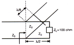
⦾ Given:
✔ Characteristic Impedance: \( Z_0 = 50\Omega \)
✔ Load Impedance: \( Z_L = 100\Omega \)
✔ Stub Length: \( \lambda/8 \) (Short-Circuited)
⦾ Step 1: Find Load Admittance \( Y_L \)
\[ Y_L = \frac{1}{Z_L} = \frac{1}{100} = 0.01 \text{ mho} \]
⦾ Step 2: Transform \( Y_L \) by \( \lambda/2 \) Section
A transmission line of length \( \lambda/2 \) does not change the admittance:
\[ Y’ = Y_L = 0.01 \text{ mho} \]
⦾ Step 3: Find the Admittance of the Short-Circuited Stub at \( \lambda/8 \)
\[ Y_{stub} = jY_0 \tan \left( \frac{2\pi}{8} \right) \]
\[ = j \cdot \frac{1}{50} \tan \left( \frac{\pi}{4} \right) \]
\[ = j \cdot 0.02 \text{ mho} \]
⦾ Step 4: Total Admittance at Junction
\[ Y = Y’ + Y_{stub} = 0.01 – j0.02 \text{ mho} \]
⦾ Final Answer: Option (a): \( 0.01 – j0.02 \) mho
Solution =
The directivity of an antenna array is a measure of how well the antenna focuses radiation in a particular direction. Adding more antenna elements to an array can increase the directivity. Here’s why:
✔ Improves the Radiation Efficiency: While adding more elements can improve the overall system efficiency, this is not the primary reason for increased directivity.
✔ Increases the Effective Area of the Antenna: Adding more elements increases the effective aperture or area of the antenna array, which directly contributes to higher directivity.
✔ Results in a Better Impedance Matching: Better impedance matching improves power transfer but does not directly affect directivity.
✔ Allows More Power to be Transmitted by the Antenna: While more elements can handle more power, this does not directly increase directivity.
The primary reason for increased directivity with more antenna elements is that it increases the effective area of the antenna, allowing it to focus the radiation more narrowly.
⦾ Final Answer: b) increases the effective area of the antenna
Solution =
The relationship between electric field lines and equipotential lines is a fundamental concept in electrostatics. Here’s the explanation:
✔ Electric Field Lines: These lines represent the direction of the electric field at any point in space. The tangent to an electric field line at any point gives the direction of the electric field at that point.
✔ Equipotential Lines: These are lines (or surfaces in three dimensions) where the electric potential is constant. No work is done in moving a charge along an equipotential line because the potential difference is zero.
⦾ Key Relationship:
Orthogonality: Electric field lines and equipotential lines are always perpendicular (orthogonal) to each other. This is because the electric field is the gradient of the electric potential, and the gradient is always perpendicular to the equipotential surfaces.
⦾ Why They Are Orthogonal:
The electric field \( \mathbf{E} \) is related to the electric potential \( V \) by:
\[ \mathbf{E} = -\nabla V \]
The gradient \( \nabla V \) points in the direction of the steepest increase of \( V \), and the electric field lines point in the direction of the steepest decrease of \( V \).
Equipotential lines are surfaces of constant \( V \), so the gradient (and thus the electric field) must be perpendicular to these surfaces.
⦾ Final Answer: c) cut each other orthogonally
Solution =
The maximum EMF induced in a rotating loop is given by:
\[ \mathcal{E}_{\text{max}} = B \cdot A \cdot \omega \]
⦾ Where:
\( B = 0.1 \, \text{T} \) (magnetic field)
\( A = \pi R^2 \) (area of the loop, with \( R = 0.5 \, \text{m} \))
\( \omega = 50 \, \text{rad/s} \) (angular velocity)
⦾ Step 1: Calculate the area of the loop
\[ A = \pi R^2 = \pi (0.5)^2 = \pi \cdot 0.25 \approx 0.785 \]
⦾ Step 2: Substituting into the formula for maximum EMF
\[ \mathcal{E}_{\text{max}} = B \cdot A \cdot \omega = (0.1) \cdot (0.785) \cdot (50) \]
⦾ Step 3: Simplify the calculation
\[ \mathcal{E}_{\text{max}} = 0.1 \cdot 0.785 \cdot 50 = 3.925 \, \text{V} \]
⦾ Answer
The closest option to the calculated value is: \[ \boxed{3.92 \, \text{V}} \]
Solution =
⦾ The magnetic force on the particle is given by:
\[ \vec{F} = q (\vec{v} \times \vec{B}) \]
⦾ Step 1: Calculate the cross product \( \vec{v} \times \vec{B} \):
\[ \vec{v} = 10^6 \hat{i}, \quad \vec{B} = 0.1 \hat{k} \] \[ \vec{v} \times \vec{B} = (10^6 \hat{i}) \times (0.1 \hat{k}) =\]\[ 10^6 \cdot 0.1 (\hat{i} \times \hat{k}) \]
Using the right-hand rule, \( \hat{i} \times \hat{k} = -\hat{j} \):
\[ \vec{v} \times \vec{B} = -10^5 \hat{j} \]
⦾ Step 2: Find the magnitude of the force:
\[ F = q |\vec{v} \times \vec{B}| \]
Substitute the values:
\[ F = (1 \times 10^{-6}) \cdot (10^5) = 0.1 \, \text{N} \]
⦾ Answer:
The magnitude of the force experienced by the particle is:
(b) 0.1 N
Solution =
⦾ Step 1: Calculate the Inductance (L)
We use the formula for inductance of a solenoid:
\[ L = \frac{\mu_0 N^2 A}{l} \]
Substitute the given values:
\[ L = \frac{(4\pi \times 10^{-7}) \cdot (1000)^2 \cdot (10^{-3})}{0.5} \]
Simplifying the expression:
\[ L = \frac{(4\pi \times 10^{-7}) \cdot 10^6 \cdot 10^{-3}}{0.5} \]
\[ L = (4\pi \times 10^{-7}) \cdot 2000 \]
Using \(\pi \approx 3.14\), we get:
\[ L = 8 \times 3.14 \times 10^{-4} = 2.512 \times 10^{-3} \, \text{H} \]
⦾ Step 2: Calculate the Energy Stored (U)
The energy stored in the magnetic field is given by the formula:
\[ U = \frac{1}{2} L I^2 \]
Substitute the values \( L = 2.512 \times 10^{-3} \, \text{H} \) and \( I = 2 \, \text{A} \):
\[ U = \frac{1}{2} \cdot 2.512 \times 10^{-3} \cdot (2)^2 \]
\[ U = \frac{1}{2} \cdot 2.512 \times 10^{-3} \cdot 4 \]
\[ U = 5.024 \times 10^{-3} \, \text{J} \]
The energy stored in the solenoid is:
\[ U = 5.024 \times 10^{-3} \, \text{J} \]
Solution =
To calculate the magnetic field at the center of a circular loop carrying a current, we use the formula:
\[ B = \frac{\mu_0 I}{2r} \]
⦾ Where:
✔ \( B \) is the magnetic field at the center of the loop.
✔ \( \mu_0 = 4\pi \times 10^{-7} \, \text{T} \cdot \text{m/A} \) is the permeability of free space.
✔ \( I = 5 \, \text{A} \) is the current through the loop.
✔ \( r = 0.1 \, \text{m} \) is the radius of the loop.
Now, substitute the given values into the formula:
\[ B = \frac{4\pi \times 10^{-7} \times 5}{2 \times 0.1} \]
Performing the calculation:
\[ B = \frac{4\pi \times 10^{-7} \times 5}{0.2} = \frac{2\pi \times 10^{-6}}{0.2} = \]\[\pi \times 10^{-5} \]
Using \( \pi \approx 3.14 \), we get:
\[ B \approx 3.14 \times 10^{-5} \, \text{T} \]
⦾ Answer:
The magnetic field at the center of the loop is approximately \( 3.14 \times 10^{-5} \, \text{T} \). Therefore, the correct answer is: (a) \( 3.14 \times 10^{-5} \, \text{T} \)
Solution =
The magnetic flux \( \Phi \) linked with a circular loop is given by the formula:
\[ \Phi = B \cdot A \cdot \cos(\theta) \]
⦾ Where:
✔ \( \Phi \) is the magnetic flux linked with the loop.
✔ \( B = 0.5 \, \text{T} \) is the magnetic field strength.
✔ \( A = \pi r^2 \) is the area of the loop, where \( r = 0.2 \, \text{m} \) is the radius of the loop.
\( \theta = 0^\circ \) is the angle between the magnetic field and the normal to the loop (since the field is perpendicular to the area).
Now, let’s calculate the area of the loop:
\[ A = \pi r^2 = \pi (0.2)^2 = 3.14 \times 0.04 =\]\[ 0.1256 \, \text{m}^2 \]
Since \( \cos(0^\circ) = 1 \), the formula for magnetic flux simplifies to:
\[ \Phi = B \cdot A = 0.5 \times 0.1256 = 0.0628 \, \text{Wb} \]
⦾ Answer:
The magnetic flux linked with the loop is \( 0.0628 \, \text{Wb} \). Therefore, the correct answer is: (b) \( 0.0628 \, \text{Wb} \)
Solution =
The magnetic field inside a solenoid is given by:
\[ B = \mu_0 n I \]
⦾ Where:
✔ \( \mu_0 = 4 \pi \times 10^{-7} \, \text{H/m} \) is the permeability of free space.
✔ \( n = 1000 \, \text{turns/m} \) is the number of turns per meter.
✔ \( I = 2 \, \text{A} \) is the current flowing through the solenoid.
⦾ Step 1: Substitute the values into the formula:
\[ B = (4 \pi \times 10^{-7}) \cdot (1000) \cdot (2) \]
⦾ Step 2: Simplify the terms:
First, calculate \( 4 \pi = 12.56 \).
Now multiply: \[ B = 12.56 \times 10^{-7} \cdot 1000 \cdot 2 \]
Simplify \( 10^{-7} \cdot 1000 = 10^{-4} \):
\[ B = 12.56 \cdot 10^{-4} \cdot 2 \]
Finally: \[ B = 25.12 \cdot 10^{-4} \, \text{T} \]
⦾ Step 3: Convert to millitesla:
\[ B = 2.512 \times 10^{-3} \, \text{T} = 2.512 \, \text{mT} \]
⦾ Final Answer:
The correct answer is: (c) \( 2.5 \times 10^{-3} \, \text{T} \)
Solution =
The energy \( U \) stored in the magnetic field of the coil is given by the formula:
\[ U = \frac{1}{2} L I^2 \]
⦾ Where:
✔ \( L = 5 \, \text{H} \) (inductance)
✔ \( I = 2 \, \text{A} \) (current)
⦾ Step 1: Substitute the values:
\[ U = \frac{1}{2} \cdot 5 \cdot (2)^2 \]
⦾ Step 2: Perform the calculation:
\[ U = \frac{1}{2} \cdot 5 \cdot 4 = 10 \, \text{J} \]
⦾ Final Answer: The energy stored in the magnetic field is: (c) \( 10 \, \text{J} \)
Solution =
⦾ Answer: (a) Resistance in an electric circuit
⦾ Explanation:
Reluctance in a magnetic circuit determines the opposition to the magnetic flux, just as resistance in an electric circuit determines the opposition to electric current. Both reluctance and resistance are proportional to their respective lengths and inversely proportional to their cross-sectional areas.
⦾ Magnetic Circuit (Reluctance):
\[ \mathcal{R} = \frac{l}{\mu A} \]
⦾ Where:
✔ \( \mathcal{R} \) is reluctance,
✔ \( l \) is the length of the magnetic path,
✔ \( \mu \) is the permeability,
✔ \( A \) is the cross-sectional area.
⦾ Electric Circuit (Resistance):
\[ R = \frac{\rho l}{A} \]
⦾ Where:
✔ \( R \) is resistance,
✔ \( \rho \) is the resistivity,
✔ \( l \) is the length of the conductor,
✔ \( A \) is the cross-sectional area.
Thus, reluctance is analogous to resistance in an electric circuit.
Solution =
⦾ Answer: (b) The flux density divided by the permeability of the medium
⦾ Explanation:
Magnetic field intensity (\(H\)) is defined as the magnetizing force that produces a magnetic field in a given medium. It is related to the magnetic flux density (\(B\)) and the permeability (\(\mu\)) of the medium through the following
⦾ equation:
\[ H = \frac{B}{\mu} \]
⦾ Where:
✔ \(H\) is the magnetic field intensity (measured in A/m),
✔ \(B\) is the magnetic flux density (measured in T),
✔ \(\mu\) is the permeability of the medium (measured in H/m).
Thus, \(H\) represents the magnetic field intensity as the ratio of flux density to the permeability of the medium.
Solution =
⦾ Answer: (a) Proportional to the product of their self-inductances
⦾ Explanation:
Mutual inductance (\(M\)) is a measure of the ability of one coil to induce an electromotive force (EMF) in another coil when the current in the first coil changes. The mutual inductance depends on:
✔ The self-inductances (\(L_1\) and \(L_2\)) of the two coils.
✔ The geometric coupling between the coils (measured by the coupling coefficient, \(k\), which ranges from 0 to 1).
The formula for mutual inductance is:
\[ M = k \sqrt{L_1 L_2} \]
⦾ Where:
✔ \(M\) is the mutual inductance,
✔ \(L_1\) and \(L_2\) are the self-inductances of the two coils,
✔ \(k\) is the coupling coefficient (\(0 \leq k \leq 1\)).
Thus, \(M\) is proportional to the product of the square roots of the self-inductances, which implies it is ultimately proportional to the product of their self-inductances.
Solution =
⦾ Answer: (d) The ability of the coil to oppose changes in the current flowing through it
⦾ Explanation:
Self-inductance (\(L\)) is a property of a coil that quantifies its ability to oppose changes in the current flowing through it. This opposition arises because the coil induces an electromotive force (EMF) in itself, according to Lenz’s Law. The self-induced EMF (\(E\)) is expressed as:
\[ E = -L \frac{dI}{dt} \]
⦾ Where:
✔ \(L\) is the self-inductance of the coil.
✔ \(\frac{dI}{dt}\) is the rate of change of current through the coil.
Thus, self-inductance is the coil’s inherent ability to resist variations in current by generating a counter EMF.
Solution =
⦾ Answer: (d) The product of magnetic field intensity and area perpendicular to it
⦾ Explanation:
Magnetic flux (\( \Phi_B \)) is a measure of the total magnetic field passing through a given area. It is mathematically defined as:
\[ \Phi_B = B \cdot A \cdot \cos \theta \]
⦾ Where:
✔ \(B\) is the magnetic field intensity (in Tesla, \(T\))
✔ \(A\) is the area through which the field lines pass (in square meters, \(m^2\))
✔ \(\theta\) is the angle between the magnetic field and the normal to the surface
When the area is perpendicular to the magnetic field (\(\theta = 0^\circ\)), \(\cos \theta = 1\), and the flux becomes:
\[ \Phi_B = B \cdot A \]
Thus, magnetic flux is the product of magnetic field intensity and the area perpendicular to it.
Solution =
⦾ Given:
✔ Area of the plates, \( A = 0.1 \, \text{m}^2 \)
✔ Separation between plates, \( d = 0.01 \, \text{m} \)
✔ Permittivity of free space, \( \varepsilon_0 = 8.85 \times 10^{-12} \, \text{F/m} \)
⦾ Formula:
The capacitance is given by:
C = \(\frac{\varepsilon_0 \cdot A}{d}\)
⦾ Calculation:
Substituting the values into the formula:
C = \(\frac{(8.85 \times 10^{-12}) \cdot 0.1}{0.01} C = 8.85 \times 10^{-11} \, \text{F}\)
⦾ Answer:
The capacitance is \( 8.85 \times 10^{-11} \, \text{F} \).
⦾ Correct Answer: (c) \( 8.85 \times 10^{-11} \, \text{F} \)
Solution =
⦾ Given:
✔ Capacitance: \( C = 10 \, \mu F = 10 \times 10^{-6} \, F \)
✔ Voltage: \( V = 100 \, V \)
⦾ Formula:
The energy stored in the capacitor is given by:
U = \( \frac{1}{2} C V^2\)
⦾ Calculation:
Substituting the values into the formula:
\( \frac{1}{2} \times (10 \times 10^{-6}) \times (100)^2 U = 0.05 \, J\)
⦾ Answer:
The energy stored in the capacitor is \( U = 0.05 \, J \).
⦾ Correct Answer: (a) \( 0.05 \, J \)
Solution =
The correct physical implication of Faraday’s Law of Induction is: (b) A changing magnetic field induces a current in a conductor.
⦾ Explanation:
Faraday’s Law states that the induced electromotive force (EMF) in a closed loop is proportional to the negative rate of change of magnetic flux through the loop. Mathematically, this is expressed as:
\[ \mathcal{E} = -\frac{d\Phi_B}{dt} \]
✔ \(\mathcal{E}\) is the induced electromotive force (EMF).
✔ \(\Phi_B\) is the magnetic flux, defined as \(\Phi_B = \int \mathbf{B} \cdot d\mathbf{A}\).
✔ \(\mathbf{B}\) is the magnetic field.
The negative sign represents Lenz’s Law, which states that the induced current opposes the change in magnetic flux that caused it.
As the magnetic flux through a conductor changes (due to a time-varying magnetic field), an EMF is generated, which can drive a current if the conductor forms a closed loop.
⦾ Why not the other options?
(a) This describes one aspect of Maxwell’s equations (specifically, the Ampère-Maxwell law), but it is not directly related to Faraday’s Law.
(c) This describes the Lorentz force, which states that a magnetic field can exert a force on a moving charge, but it is not related to Faraday’s Law.
(d) A changing electric field does not produce an electric force. Instead, it can produce a magnetic field (another aspect of Maxwell’s equations).
Solution =
(c) The potential is determined only by the charge distribution on the sphere.
⦾ Explanation:
✔ Conducting Sphere in an External Field:
A conducting sphere placed in an external electric field will experience a redistribution of its free charges. This redistribution ensures that the electric field inside the conductor is zero and the potential on its surface is constant.
✔ Potential Outside the Sphere:
Outside the sphere, the total potential at any point is the sum of the potential due to the charge Q on the sphere and the potential due to the external field.
However, the induced charge on the surface of the conducting sphere cancels the effect of the external field, leaving the potential at any point outside the sphere dependent solely on the charge Q distributed over the sphere.
✔ Why the Potential Remains Unaffected:
The conducting sphere redistributes its charge to maintain equilibrium, ensuring that the potential outside the sphere depends only on the total charge Q. This behavior stems from the unique properties of conductors and the principle of superposition in electrostatics.
⦾ Why Not the Other Options?
(a) While a conducting sphere does shield the external field within its interior, this does not explain why the potential at a point outside the sphere remains unaffected.
(b) The induced charge does cancel the external field, but this is a mechanism rather than a reason why the potential outside depends only on the charge Q.
(d) The sphere redistributes its charge to maintain constant potential on its surface, but this is a statement about the surface potential, not the reason for the potential outside being unaffected by the external field.
Solution =
⦾ We are given the incident electric field:
\[ \vec{E_i} = 24\cos\left(3 \times 10^8 t + \beta y\right) \hat{a}_x \, \text{V/m} \] The wave is incident normally on a lossless medium with \(\mu = \mu_0\) and \(\varepsilon = 9\varepsilon_0\) for \(y \geq 0\).
⦾ Step 1: Determine the wave number \(\beta\) in free space
The wave number \(\beta\) in free space is given by:
\[ \beta = \frac{\omega}{c} = \frac{3 \times 10^8}{3 \times 10^8} = 1 \, \text{rad/m} \] ⦾ Step 2: Calculate the intrinsic impedances
The intrinsic impedance of free space (\(\eta_1\)) and the medium (\(\eta_2\)) are:
\[ \eta_1 = \sqrt{\frac{\mu_0}{\varepsilon_0}} = 120\pi \, \Omega \] \[ \eta_2 = \sqrt{\frac{\mu_0}{9\varepsilon_0}} = \frac{120\pi}{3} = 40\pi \, \Omega \] ⦾ Step 3: Determine the reflection coefficient \(\Gamma\)
The reflection coefficient at the boundary is:
\[ \Gamma = \frac{\eta_2 – \eta_1}{\eta_2 + \eta_1} = \frac{40\pi – 120\pi}{40\pi + 120\pi} = \frac{-80\pi}{160\pi} \]\[= -0.5 \] ⦾ Step 4: Calculate the reflected electric field \(\vec{E_r}\)
The reflected electric field is:
\[ \vec{E_r} = \Gamma \vec{E_i} \]\[= -0.5 \times 24\cos\left(3 \times 10^8 t + y\right) \hat{a}_x \]\[= -12\cos\left(3 \times 10^8 t + y\right) \hat{a}_x \, \text{V/m} \] ⦾ Step 5: Determine the reflected magnetic field \(\vec{H_r}\)
The relationship between the electric and magnetic fields in a plane wave is:
\[ \vec{H} = \frac{1}{\eta} \hat{a}_k \times \vec{E} \] For the reflected wave, the direction of propagation is in the \(-y\) direction. Thus:
\[ \vec{H_r} = \frac{1}{\eta_1} \hat{a}_y \times \vec{E_r} \] Substituting the values:
\[ \vec{H_r} = \frac{1}{120\pi} \hat{a}_y \times \]\[\left(-12\cos\left(3 \times 10^8 t + y\right) \hat{a}_x\right) \] The cross product \(\hat{a}_y \times \hat{a}_x = -\hat{a}_z\), so:
\[ \vec{H_r} = \frac{1}{120\pi} \times (-12) \]\[\times (-\hat{a}_z) \cos\left(3 \times 10^8 t + y\right) \] Simplifying:
\[ \vec{H_r} = \frac{12}{120\pi} \hat{a}_z \cos\left(3 \times 10^8 t + y\right) \]\[= \frac{1}{10\pi} \cos\left(3 \times 10^8 t + y\right) \hat{a}_z \, \text{A/m} \] ⦾ Step 6: Compare with the given options
The reflected magnetic field component is:
\[ \frac{1}{10\pi} \cos\left(3 \times 10^8 t + y\right) \hat{a}_z \, \text{A/m} \] ⦾ The correct option is: \[ \boxed{\text{a) } \frac{1}{10\pi}\cos\left(3 \times 10^8 t + y\right)\hat{a}_x \, \text{A/m}} \]
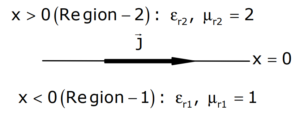
In Region-1 (\(x < 0\)): \(\varepsilon_{r1} = 1\), \(\mu_{r1} = 1\)
In Region-2 (\(x > 0\)): \(\varepsilon_{r2} = 2\), \(\mu_{r2} = 2\)
The magnetic field in Region-1 at \(x = 0\) is: \( \overrightarrow{H_1} = 3\hat{u}_x + 30\hat{u}_y \text{ A/m} \) Determine the magnetic field \(\overrightarrow{H_2}\) in Region-2 at \(x = 0^+\).
(A) \(\overrightarrow{H_2} = 1.5\hat{u}_x + 30\hat{u}_y – 10\hat{u}_z\) A/m
(B) \(\overrightarrow{H_2} = 3\hat{u}_x + 30\hat{u}_y – 10\hat{u}_z\) A/m
(C) \(\overrightarrow{H_2} = 1.5\hat{u}_x + 40\hat{u}_y\) A/m
(D) \(\overrightarrow{H_2} = 3\hat{u}_x + 30\hat{u}_y + 10\hat{u}_z\) A/m
Solution =
⦾ Given:
A current sheet \(\vec{J} = 10\hat{u}_y\) A/m lies on the dielectric interface \(x = 0\).
✔ In Region-1 (\(x < 0\)): \(\varepsilon_{r1} = 1\), \(\mu_{r1} = 1\).
✔ In Region-2 (\(x > 0\)): \(\varepsilon_{r2} = 2\), \(\mu_{r2} = 2\).
The magnetic field in Region-1 at \(x = 0\) is \(\overrightarrow{H_1} = 3\hat{u}_x + 30\hat{u}_y\) A/m.
Solution:
⦾ Step 1: Apply Boundary Conditions
At the interface \(x = 0\), the boundary conditions for the magnetic field are: \[ \overrightarrow{H_{2t}} – \overrightarrow{H_{1t}} = \vec{J} \times \hat{n} \] where \(\hat{n}\) is the unit normal vector pointing from Region-1 to Region-2 (\(\hat{u}_x\)).
⦾ Step 2: Calculate the Tangential Components
Given \(\overrightarrow{H_1} = 3\hat{u}_x + 30\hat{u}_y\) A/m, the tangential components are: \[ \overrightarrow{H_{1t}} = 30\hat{u}_y \]
⦾ Step 3: Apply the Boundary Condition
Using the boundary condition: \[ \overrightarrow{H_{2t}} – 30\hat{u}_y = -10\hat{u}_z \] Therefore: \[ \overrightarrow{H_{2t}} = 30\hat{u}_y – 10\hat{u}_z \]
⦾ Step 4: Determine the Normal Component
The normal component of \(\overrightarrow{H}\) is continuous across the interface: \[ H_{2x} = H_{1x} = 3\hat{u}_x \]
⦾ Step 5: Combine Components
Combining the tangential and normal components, the magnetic field in Region-2 at \(x = 0^+\) is: \[ \overrightarrow{H_2} = 3\hat{u}_x + 30\hat{u}_y – 10\hat{u}_z \text{ A/m} \]
⦾ Final Answer
The correct option is: \[ \overrightarrow{H_2} = 3\hat{u}_x + 30\hat{u}_y – 10\hat{u}_z \text{ A/m} \]
Solution =
To calculate the gain of a parabolic dish antenna, we use the formula:
\[ G = \eta \left( \frac{\pi D}{\lambda} \right)^2 \]
⦾ where:
✔ \( G \) is the gain of the antenna (in linear scale),
✔ \( \eta \) is the efficiency of the antenna (70% or 0.7),
✔ \( D \) is the diameter of the dish (1 meter),
✔ \( \lambda \) is the wavelength of the signal.
First, calculate the wavelength (\( \lambda \)) at 20 GHz:
\[ \lambda = \frac{c}{f} \]
where \( c \) is the speed of light (\( 3 \times 10^8 \) m/s) and \( f \) is the frequency (20 GHz or \( 20 \times 10^9 \) Hz).
\[ \lambda = \frac{3 \times 10^8}{20 \times 10^9} = 0.015 \text{ meters} \]
Now, substitute the values into the gain formula:
\[ G = 0.7 \left( \frac{\pi \times 1}{0.015} \right)^2 \]
Calculate the term inside the parentheses:
\[ \frac{\pi \times 1}{0.015} \approx 209.44 \]
Now, square this value:
\[ 209.44^2 \approx 43860 \]
Multiply by the efficiency:
\[ G = 0.7 \times 43860 \approx 30702 \]
To convert this gain from linear scale to decibels (dB), use the formula:
\[ G_{\text{dB}} = 10 \log_{10}(G) \]
\[ G_{\text{dB}} = 10 \log_{10}(30702) \approx 10 \times 4.487 \]\[\approx 44.87 \text{ dB} \]
Rounding to the nearest whole number, the gain is approximately 45 dB.
⦾ Final Answer: d) 45 dB
Solution =
For a Hertz dipole antenna, the half-power beamwidth (HPBW) in the E-plane is a well-known characteristic. The E-plane is the plane that contains the electric field vector and the direction of maximum radiation.
⦾ For a Hertz dipole antenna:
The half-power beamwidth (HPBW) in the E-plane is 90°.
This means that the angular width between the points where the radiation intensity falls to half of its maximum value is 90°.
⦾ Final Answer: c) 90°
Solution =
⦾ We are given:
✔ Electric field on the surface of the conductor: \( E = 2 \, \text{V/m} \)
✔ Permittivity of the surrounding medium (water): \( \epsilon = 80 \epsilon_0 \)
✔ \( \epsilon_0 = \frac{10^9}{36 \pi} \, \text{F/m} \)
The surface charge density \( \sigma \) is related to the electric field by the formula:
\[ E = \frac{\sigma}{\epsilon} \]
Rearranging for \( \sigma \):
\[ \sigma = \epsilon E \]
Substitute \( \epsilon \) and \( E \):
\[ \epsilon = 80 \epsilon_0 = 80 \times \frac{10^9}{36 \pi} \]
Thus,
\[ \sigma = \left( 80 \times \frac{10^9}{36 \pi} \right) \times 2 \]
Calculating the value:
\[ \sigma \approx 1.41 \times 10^{-9} \, \text{C/m}^2 \]
⦾ Final Answer: \( \sigma = 1.41 \times 10^{-9} \, \text{C/m}^2 \)
The correct option is: (d).
Solution =
We solve this using the Divergence Theorem: \[ \iint_{S} \vec{F} \cdot \hat{n} \, dS = \iiint_{V} (\nabla \cdot \vec{F}) \, dV \]
⦾ Step 1: Define the vector field
The given vector field is:
\[ \vec{F} = 3 \vec{r} \] where \(\vec{r} = (x, y, z)\).
⦾ Step 2: Compute the divergence of \(\vec{F}\)
The divergence of \(\vec{F}\) is:
\[ \nabla \cdot \vec{F} = \nabla \cdot (3 \vec{r}) = 3 (\nabla \cdot \vec{r}) \]
For \(\vec{r} = (x, y, z)\), we know:
\[ \nabla \cdot \vec{r} = \frac{\partial x}{\partial x} + \frac{\partial y}{\partial y} + \frac{\partial z}{\partial z} \]\[ = 1 + 1 + 1 = 3 \]
Thus:
\[ \nabla \cdot \vec{F} = 3 \cdot 3 = 9 \]
⦾ Step 3: Apply the Divergence Theorem
Using the Divergence Theorem, we substitute into the volume integral:
\[ \iint_{S} \vec{F} \cdot \hat{n} \, dS = \iiint_{V} (\nabla \cdot \vec{F}) \, dV \]\[ = \iiint_{V} 9 \, dV \]
Since the volume integral of \(9\) over \(V\) is:
\[ \iiint_{V} 9 \, dV = 9 \cdot V \]
we find:
\[ \iint_{S} \vec{F} \cdot \hat{n} \, dS = 9V \]
⦾ Final Answer:
The value of the surface integral is:
\[ \boxed{9V} \]

(A) uniform and depends only on
(B) uniform and depends only on b
(C) uniform and depends on both b and d
(D) non uniform
Solution =
Magnetic Field Inside a Wire with a Hole This problem involves the superposition principle in electromagnetism, specifically the field distribution inside a conductor with a missing section (a hole).
⦾ Conceptual Explanation:
1. Current Distribution in the Wire:
The infinitely long conductor has a uniform current density \( j \). If no hole were present, the magnetic field inside the conductor could be derived from Ampère’s law.
2. Effect of the Hole:
The hole is created at a distance \( d \) from the center, effectively removing a portion of the current-carrying conductor. This scenario can be analyzed using superposition, where the situation is treated as:
✔ A full wire with uniform \( j \), producing a field \( B_{\text{full}} \).
✔ A “negative” current (opposite in direction to the original) of the same current density \( j \) within the region of the hole. This produces a field \( B_{\text{hole}} \).
3. Resulting Magnetic Field:
The combined field inside the hole turns out to be uniform and depends on both \( b \) (hole radius) and \( d \) (distance from the center).
The field inside a cylindrical cavity in a uniformly magnetized region behaves similarly to a uniform field in a homogeneous medium.
⦾ Answer:
(c) Uniform and depends on both \( b \) and \( d \).
Solution =
⦾ The correct answer is: a) Helical motion in the \( \hat{z} \) direction.
⦾ Explanation:
1. Magnetic Force and Motion: A charged particle moving in a magnetic field experiences a force given by the Lorentz force equation:
\[ \mathbf{F} = q (\mathbf{v} \times \mathbf{B}) \]
2. Components of Velocity:
The particle has an initial velocity with components in the \( \hat{x} \) and \( \hat{z} \) directions:
\[ \mathbf{v} = \hat{x}v_x + \hat{z}v_z \]
The magnetic field is in the \( \hat{z} \) direction:
\[ \mathbf{B} = \hat{z}B \]
3. Effect of Magnetic Field:
✔ The component of velocity in the \( \hat{z} \) direction (\( v_z \)) is parallel to the magnetic field and thus does not experience any magnetic force. This means the particle will continue to move with constant velocity \( v_z \) in the \( \hat{z} \) direction.
✔ The component of velocity in the \( \hat{x} \) direction (\( v_x \)) is perpendicular to the magnetic field. This component will experience a force causing circular motion in the plane perpendicular to \( \mathbf{B} \), which is the xy-plane.
4. Resulting Motion:
The combination of the circular motion in the xy-plane and the linear motion in the \( \hat{z} \) direction results in a helical trajectory.
The axis of the helix is along the \( \hat{z} \) direction.
Therefore, the particle’s eventual trajectory is a helical motion in the \( \hat{z} \) direction.
Solution =
⦾ Given the vector function:
\[ F = \hat{a}_x (4y – k_1z) + \hat{a}_y (k_2x – 3z) + \]\[\hat{a}_z (k_3y + 2z) \] To determine the values of the constants \( k_1 \), \( k_2 \), and \( k_3 \) for \( F \) to be irrotational, we compute the curl of \( F \):
\[ \nabla \times F = \hat{a}_x \left( \frac{\partial F_z}{\partial y} – \frac{\partial F_y}{\partial z} \right) +\]\[ \hat{a}_y \left( \frac{\partial F_x}{\partial z} – \frac{\partial F_z}{\partial x} \right) + \hat{a}_z \left( \frac{\partial F_y}{\partial x} – \frac{\partial F_x}{\partial y} \right) \] Compute each component of the curl:
For the \( \hat{a}_x \) component: \[ \frac{\partial F_z}{\partial y} – \frac{\partial F_y}{\partial z} \]\[= \frac{\partial (k_3y + 2z)}{\partial y} – \frac{\partial (k_2x – 3z)}{\partial z} \]\[= k_3 – (-3) = k_3 + 3 \]
For the \( \hat{a}_y \) component: \[ \frac{\partial F_x}{\partial z} – \frac{\partial F_z}{\partial x} \]\[= \frac{\partial (4y – k_1z)}{\partial z} – \frac{\partial (k_3y + 2z)}{\partial x} \]\[= -k_1 – 0 = -k_1 \]
For the \( \hat{a}_z \) component: \[ \frac{\partial F_y}{\partial x} – \frac{\partial F_x}{\partial y} \]\[= \frac{\partial (k_2x – 3z)}{\partial x} – \frac{\partial (4y – k_1z)}{\partial y} \]\[= k_2 – 4 \]
For \( F \) to be irrotational, each component of the curl must be zero:
\[ k_3 + 3 = 0 \quad \Rightarrow \quad k_3 = -3 \] \[ -k_1 = 0 \quad \Rightarrow \quad k_1 = 0 \] \[ k_2 – 4 = 0 \quad \Rightarrow \quad k_2 = 4 \] Thus, the values of the constants are:
\[ k_1 = 0, \quad k_2 = 4, \quad k_3 = -3 \] However, The correct option is: a) 0.0, 4.0, -3.0
Solution =
⦾ Given:
✔ Charge \( q = 3 \, \text{nC} = 3 \times 10^{-9} \, \text{C} \)
✔ Position of the real charge: \((0, 0, 0.5) \, \text{m}\)
✔ Position of the image charge: \((0, 0, -0.5) \, \text{m}\)
✔ Point where the E-field is calculated: \((0, 0, 0.3) \, \text{m}\)
✔ Permittivity of free space: \(\varepsilon_0 = 8.85 \times 10^{-12} \, \text{F/m}\)
⦾ Step 1: Distance from the real charge to the point
The distance \( r_1 \) from the real charge \((0, 0, 0.5)\) to the point \((0, 0, 0.3)\) is: \[ r_1 = |0.3 – 0.5| = 0.2 \, \text{m} \]
⦾ Step 2: Distance from the image charge to the point
The distance \( r_2 \) from the image charge \((0, 0, -0.5)\) to the point \((0, 0, 0.3)\) is: \[ r_2 = |0.3 – (-0.5)| = 0.8 \, \text{m} \]
⦾ Step 3: Electric field due to the real charge
The electric field \( E_1 \) due to the real charge is: \[ E_1 = \frac{1}{4 \pi \varepsilon_0} \frac{q}{r_1^2} \] Substitute the values: \[ E_1 = \frac{1}{4 \pi \times 8.85 \times 10^{-12}} \frac{3 \times 10^{-9}}{(0.2)^2} \] \[ E_1 = 8.99 \times 10^9 \times \frac{3 \times 10^{-9}}{0.04} \] \[ E_1 = 674.25 \, \text{V/m} \]
⦾ Step 4: Electric field due to the image charge
The electric field \( E_2 \) due to the image charge is: \[ E_2 = \frac{1}{4 \pi \varepsilon_0} \frac{-q}{r_2^2} \] Substitute the values: \[ E_2 = \frac{1}{4 \pi \times 8.85 \times 10^{-12}} \frac{-3 \times 10^{-9}}{(0.8)^2} \] \[ E_2 = 8.99 \times 10^9 \times \frac{-3 \times 10^{-9}}{0.64} \] \[ E_2 = -42.14 \, \text{V/m} \]
⦾ Step 5: Total Z-component of the electric field
The total \(Z\)-component of the electric field is the sum of \( E_1 \) and \( E_2 \): \[ E_{\text{total}} = E_1 + E_2 \] \[ E_{\text{total}} = 674.25 \, \text{V/m} – 42.14 \, \text{V/m} \] \[ E_{\text{total}} = 632.11 \, \text{V/m} \]
⦾ The correct option is: \[ \boxed{a) \, 632.11 \, \text{V/m}} \]
Solution =
To determine the frequency at which the conduction current equals the displacement current in a material, we use the following relationship:
\[ \sigma = \omega \epsilon \]
⦾ Where:
✔ \(\sigma\) is the conductivity of the material.
✔ \(\omega\) is the angular frequency.
✔ \(\epsilon\) is the permittivity of the material.
⦾ Given:
✔ Conductivity, \(\sigma = 10^{-2} \, \text{mho/m}\)
✔ Relative permittivity, \(\epsilon_r = 4\)
✔ Permittivity of free space, \(\epsilon_0 = 8.854 \times 10^{-12} \, \text{F/m}\)
First, calculate the permittivity of the material:
\[ \epsilon = \epsilon_r \epsilon_0 = 4 \times 8.854 \times 10^{-12} \, \text{F/m} \]\[= 3.5416 \times 10^{-11} \, \text{F/m} \]
Next, set the conduction current equal to the displacement current:
\[ \sigma = \omega \epsilon \]
\[ 10^{-2} = \omega \times 3.5416 \times 10^{-11} \]
Solve for \(\omega\):
\[ \omega = \frac{10^{-2}}{3.5416 \times 10^{-11}} \]\[\approx 2.824 \times 10^8 \, \text{rad/s} \]
Convert angular frequency to frequency in Hz:
\[ f = \frac{\omega}{2\pi} = \frac{2.824 \times 10^8}{2\pi} \]\[\approx 4.5 \times 10^7 \, \text{Hz} = 45 \, \text{MHz} \]
Therefore, the correct answer is: a) 45 MHz
Solution =
The penetration depth (\(\delta\)) of an electromagnetic wave in a conductive medium is given by the formula:
\[ \delta = \frac{1}{\sqrt{\pi f \mu \sigma}} \]
⦾ where:
✔ \( f \) is the frequency,
✔ \( \mu \) is the permeability of the medium,
✔ \( \sigma \) is the conductivity of the medium.
Since penetration depth is inversely proportional to the square root of the frequency:
\[ \delta \propto \frac{1}{\sqrt{f}} \]
⦾ Given Data:
✔ Initial frequency \( f_1 = 2 \) MHz
✔ Initial penetration depth \( \delta_1 = 30 \) cm
✔ New frequency \( f_2 = 8 \) MHz
⦾ Using the proportionality:
\[ \frac{\delta_2}{\delta_1} = \sqrt{\frac{f_1}{f_2}} \]
\[ \delta_2 = \delta_1 \times \sqrt{\frac{2}{8}} \]
\[ \delta_2 = 30 \times \sqrt{\frac{1}{4}} \]
\[ \delta_2 = 30 \times \frac{1}{2} = 15 \text{ cm} \]
⦾ Final Answer: \( \delta_2 = 15 \) cm (Option b)
Solution =
The magnetic field intensity vector of the plane wave is given by: \( H(x,t)\)
\(= 15 \sin(60000t + 0.004x + 10) \, \hat{a}_y\)
The general form of a plane wave propagating in the \( x \)-direction is:
\[ H(x,t) = H_0 \sin(\omega t + kx + \phi) \]
⦾ From the given equation:
\[ \omega = 60000 \, \text{rad/s}, \quad k = 0.004 \, \text{rad/m} \]
The phase velocity \( v_p \) is calculated as:
\[ v_p = \frac{\omega}{k} = \frac{60000}{0.004} = 1.5 \times 10^7 \, \text{m/s} \]
⦾ Therefore, the correct answer is:
a) \(1.5 \times 10^7 \, \text{m/s}\)
Solution =
⦾ Correct Answer: (B) Zero electric field along the direction of propagation
✔ In a waveguide, TE (Transverse Electric) modes are characterized by having the electric field (E-field) entirely transverse to the direction of propagation.
✔ This means that the electric field component in the direction of propagation (Ez) is zero. However, the magnetic field (Hz) can have a component along the direction of propagation.
✔ TE modes are often used in waveguides to efficiently transmit high-frequency signals with minimal losses.
Thus, the defining characteristic of TE modes is that there is no electric field along the direction of propagation.
Solution =
In a region of space, where the permittivity \( \epsilon \) varies with the electric field \( E \) as:
\[ \epsilon(E) = \epsilon_0 \left( 1 + \alpha E^2 \right) \]
The relationship between the electric displacement field \( D \) and the electric field \( E \) is given by:
\[ D = \epsilon(E) E \]
Substituting the expression for \( \epsilon(E) \), we get the electric displacement field \( D \) as:
\[ D = \epsilon_0 \left( 1 + \alpha E^2 \right) E \]
⦾ Where:
✔ \( \epsilon_0 \) is the permittivity of free space
✔ \( \alpha \) is a constant
✔ \( E \) is the electric field
Solution =
⦾ We are given:
✔ Electric field amplitude, \( E_0 = 2 \, \text{V/m} \)
✔ Relative permittivity of the medium, \( \varepsilon_r = 4 \)
✔ The medium is nonmagnetic (\( \mu_r = 1 \)) and lossless (\( \sigma = 0 \))
⦾ Step 1: Calculate the intrinsic impedance of the medium
The intrinsic impedance \( \eta \) of the medium is given by:
\[ \eta = \sqrt{\frac{\mu}{\varepsilon}} \] For a nonmagnetic medium, \( \mu = \mu_0 \), and the permittivity \( \varepsilon = \varepsilon_r \varepsilon_0 \). Substituting these values:
\[ \eta = \sqrt{\frac{\mu_0}{4 \varepsilon_0}} = \frac{\eta_0}{\sqrt{4}} = \frac{120\pi}{2} = 60\pi \, \Omega \] where \( \eta_0 = 120\pi \, \Omega \) is the intrinsic impedance of free space.
⦾ Step 2: Calculate the time-average power density vector
The time-average power density vector \( \vec{S}_{\text{avg}} \) for a plane EM wave is given by:
\[ \vec{S}_{\text{avg}} = \frac{1}{2} \frac{E_0^2}{\eta} \hat{a}_k \] where \( \hat{a}_k \) is the direction of propagation. The magnitude of the time-average power density is:
\[ |\vec{S}_{\text{avg}}| = \frac{1}{2} \frac{E_0^2}{\eta} \] Substituting the values \( E_0 = 2 \, \text{V/m} \) and \( \eta = 60\pi \, \Omega \):
\[ |\vec{S}_{\text{avg}}| = \frac{1}{2} \frac{(2)^2}{60\pi} = \frac{1}{2} \frac{4}{60\pi} = \frac{2}{60\pi} \]\[= \frac{1}{30\pi} \, \text{W/m}^2 \] ⦾ Step 3: Match with the given options
The magnitude of the time-average power density vector is:
\[ \boxed{\frac{1}{30\pi} \, \text{W/m}^2} \] ⦾ Final Answer:
The correct option is a) \(\frac{1}{30\pi}\).
Solution =
For a transmission line to be distortionless, the following condition must be satisfied:
\[ \frac{R}{L} = \frac{G}{C} \]
⦾ Where:
✔ \( R \) is the resistance per unit length,
✔ \( L \) is the inductance per unit length,
✔ \( G \) is the conductance per unit length,
✔ \( C \) is the capacitance per unit length.
This condition ensures that the line’s attenuation and phase shift are uniform across all frequencies, preventing distortion.
Now, let’s analyze the given options:
✔ \( RL = \frac{1}{GC} \) – This does not match the required condition.
✔ \( RL = GC \) – This does not match the required condition.
✔ \( LG = RC \) – Rearranging this gives \( \frac{R}{L} = \frac{G}{C} \), which matches the required condition.
✔ \( RG = LC \) – This does not match the required condition.
⦾ Therefore, the correct answer is: c) \( LG = RC \)
Solution =
To determine the intrinsic impedance of the dielectric material, we use the given information about the electric field maxima and minima.
An electromagnetic wave propagates in free space and is incident normally on a dielectric slab. The dielectric material is lossless and non-magnetic. The maximum electric field (\(E_{\text{max}}\)) is 5 times the minimum electric field (\(E_{\text{min}}\)).
The ratio of the maximum to minimum electric field in a standing wave pattern is given by the standing wave ratio (SWR):
\[ \text{SWR} = \frac{E_{\text{max}}}{E_{\text{min}}} \]
Given \(E_{\text{max}} = 5E_{\text{min}}\), the SWR is 5.
The intrinsic impedance of free space (\(\eta_0\)) is \(120\pi \, \Omega\). The intrinsic impedance of the dielectric material (\(\eta\)) can be found using the relationship:
\[ \text{SWR} = \frac{\eta_0}{\eta} \]
Rearranging for \(\eta\):
\[ \eta = \frac{\eta_0}{\text{SWR}} = \frac{120\pi}{5} = 24\pi \, \Omega \]
Therefore, the intrinsic impedance of the dielectric material is:
d) 24πΩ
(A) \( \begin{bmatrix} -\frac{1}{2} & \frac{1}{2} \ \frac{1}{2} & -\frac{1}{2} \end{bmatrix} \)
(B) \( \begin{bmatrix} 0 & 1 \ 1 & 0 \end{bmatrix} \)
(C) \( \begin{bmatrix} \frac{1}{3} & \frac{2}{3} \ \frac{2}{3} & \frac{1}{3} \end{bmatrix} \)
(D) \( \begin{bmatrix} \frac{1}{4} & -\frac{3}{4} \ -\frac{3}{4} & \frac{1}{4} \end{bmatrix} \)
Solution =
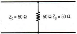
⦾ Given:
✔ Shunt Load: \( 50\Omega \)
✔ Characteristic Impedance: \( Z_0 = 50\Omega \)
✔ Transmission line terminated with \( 50\Omega \) at both ends (matched line).
⦾ Step 1: Understanding the Scattering Matrix
The S-matrix describes how an incident wave interacts with the network, including reflections and transmissions between ports.
⦾ Step 2: Condition of a Matched System
Since the transmission line is matched at both ends:
✔ No reflections occur, so: \[ S_{11} = S_{22} = 0 \]
✔ The wave is fully transmitted from port 1 to port 2 and vice versa: \[ S_{12} = S_{21} = 1 \]
⦾ Step 3: Final S-Matrix
Thus, the S-matrix is:
\[ S = \begin{bmatrix} 0 & 1 \\ 1 & 0 \end{bmatrix} \]
⦾ Step 4: Correct Answer
Comparing with the given answer choices, the correct choice is:
\[ \boxed{\text{Option (b)}} \]
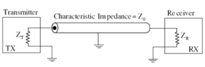
Which one of the following statements is TRUE about the distortion of the received signal due to impedance mismatch?
(A) The signal gets distorted if \( Z_R \neq Z_0 \), irrespective of the value of \( Z_T \).
(B) The signal gets distorted if \( Z_T \neq Z_0 \), irrespective of the value of \( Z_R \).
(C) Signal distortion implies impedance mismatch at both ends: \( Z_T \neq Z_0 \) and \( Z_R \neq Z_0 \).
(D) Impedance mismatches do not result in signal distortion but reduce power transfer efficiency.
Solution =
For distortion-less signal transmission, there must be a perfect impedance match at both the transmitting and receiving ends.
If either \( Z_R \) or \( Z_T \) is matched with \( Z_0 \), the signal traveling on the line will be completely absorbed at that point, preventing reflections. However, when both ends are mismatched, multiple reflections occur, leading to signal distortion.
For signal distortion to occur, both conditions must be met:
\[ Z_T \neq Z_0 \] \[ Z_R \neq Z_0 \] Thus, the correct answer is:
⦾ Option (c): “Signal distortion implies impedance mismatch at both ends: \( Z_T \neq Z_0 \) and \( Z_R \neq Z_0 \).”
Solution =
To determine the cut-off frequency of a rectangular waveguide, we use the formula for the cut-off frequency \( f_c \) for the dominant mode \( TE_{10} \):
\[ f_c = \frac{c}{2a} \]
⦾ where:
✔ \( c \) is the speed of light in vacuum (\( 3 \times 10^8 \, \text{m/s} \)),
✔ \( a \) is the wider dimension of the waveguide.
Given the dimensions of the waveguide:
✔ \( a = 1 \, \text{cm} = 0.01 \, \text{m} \),
✔ \( b = 0.5 \, \text{cm} = 0.005 \, \text{m} \).
The dominant mode \( TE_{10} \) depends on the wider dimension \( a \).
⦾ Substituting the values:
\[ f_c = \frac{3 \times 10^8}{2 \times 0.01} = \frac{3 \times 10^8}{0.02} \]\[= 15 \times 10^9 \, \text{Hz} = 15 \, \text{GHz} \]
Thus, the cut-off frequency is 15 GHz.
⦾ Final Answer:
\[ \boxed{d) \ 15 \, \text{GHz}} \]
Solution =
When a TEM (Transverse Electromagnetic) wave is incident normally upon a perfect conductor, the boundary conditions at the surface of the conductor dictate the behavior of the electric (\( \mathbf{E} \)) and magnetic (\( \mathbf{H} \)) fields.
⦾ Boundary Conditions for a Perfect Conductor:
✔ Electric Field (\( \mathbf{E} \)): The tangential component of the electric field must be zero at the surface of a perfect conductor.
This means the electric field is minimum (zero) at the boundary.
✔ Magnetic Field (\( \mathbf{H} \)): The tangential component of the magnetic field is maximum at the surface of a perfect conductor.
This means the magnetic field is maximum at the boundary.
⦾ Explanation:
– The perfect conductor reflects the incident wave, creating a standing wave pattern. – At the boundary, the electric field cancels out due to the reflection (minimum or zero). – The magnetic field, however, doubles at the boundary due to the superposition of the incident and reflected waves (maximum).
⦾ Correct Answer:
The electric field (\( \mathbf{E} \)) is minimum, and the magnetic field (\( \mathbf{H} \)) is maximum at the boundary.
\[ \boxed{c) \ \text{minimum and maximum}} \]
(A)
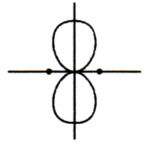 (B)
(B) 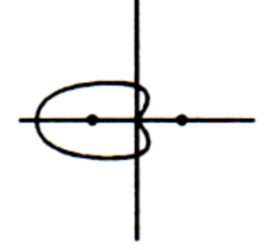
(C)
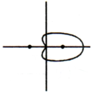 (D)
(D) 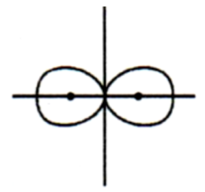
Solution =
⦾ Correct Answer = A
There will be no pattern in E-plane, only in H-Plane.
Solution =
To determine the voltage standing wave ratio (VSWR) and the reflection coefficient in an ideal transmission line with a matched load, let’s analyze the situation step by step.
⦾ Key Concepts:
✔ Matched Load: A matched load means that the load impedance \( Z_L \) is equal to the characteristic impedance \( Z_0 \) of the transmission line. In this case, there is no reflection of the signal at the load.
✔ Reflection Coefficient (\( \Gamma \)): The reflection coefficient is a measure of how much of the signal is reflected back from the load. It is given by: \[ \Gamma = \frac{Z_L – Z_0}{Z_L + Z_0} \] For a matched load (\( Z_L = Z_0 \)): \[ \Gamma = \frac{Z_0 – Z_0}{Z_0 + Z_0} = 0 \]
✔ Voltage Standing Wave Ratio (VSWR): The VSWR is a measure of the standing wave pattern on the transmission line and is given by: \[ \text{VSWR} = \frac{1 + |\Gamma|}{1 – |\Gamma|} \] For a matched load (\( \Gamma = 0 \)): \[ \text{VSWR} = \frac{1 + 0}{1 – 0} = 1 \]
⦾ Analysis:
✔ Reflection Coefficient: In a matched load condition, the reflection coefficient \( \Gamma \) is zero because there is no reflection.
✔ VSWR: With no reflection (\( \Gamma = 0 \)), the VSWR is 1, indicating no standing waves and a perfectly matched line.
⦾ Final Answer: d) one and zero
Solution =
⦾ Given:
\[ \mathbf{E} = x\mathbf{u_x} + y\mathbf{u_y} + z\mathbf{u_z} \]
The potential difference \(V_{YX}\) is given by:
\[ V_{YX} = – \int_X^Y \mathbf{E} \cdot d\mathbf{l} \]
Substituting \(\mathbf{E} \cdot d\mathbf{l} = x dx + y dy + z dz\), the integral becomes:
\[ V_{YX} = – \int_X^Y (x dx + y dy + z dz) \]
⦾ Step 1: Evaluate the integral for \(x\):
\[ \int_X^Y x dx = \int_{x=2}^{x=1} x dx = \left[\frac{x^2}{2}\right]_2^1 =\]\[ \frac{1^2}{2} – \frac{2^2}{2} = -\frac{3}{2} \]
⦾ Step 2: Evaluate the integral for \(y\):
\[ \int_X^Y y dy = \int_{y=0}^{y=2} y dy = \left[\frac{y^2}{2}\right]_0^2 =\]\[ \frac{2^2}{2} – \frac{0^2}{2} = 2 \]
⦾ Step 3: Evaluate the integral for \(z\):
\[ \int_X^Y z dz = \int_{z=0}^{z=3} z dz = \left[\frac{z^2}{2}\right]_0^3 =\]\[ \frac{3^2}{2} – \frac{0^2}{2} = \frac{9}{2} \]
⦾ Step 4: Combine the results:
\[ V_{YX} = – \left(-\frac{3}{2} + 2 + \frac{9}{2}\right) \]
Simplify:
\[ V_{YX} = – \left(\frac{-3}{2} + \frac{4}{2} + \frac{9}{2}\right) = – \left(\frac{10}{2}\right) \]\[= -5 \, \text{V} \]
⦾ Final Answer:
\[ V_{YX} = -5 \, \text{V} \]
The correct option is: (c) -5 volts.
Solution =
⦾ We are given the surface integral:
\[ \iint_S \mathbf{F} \cdot \hat{n} \, dS \] where \( \mathbf{F} = x^2 \hat{i} + y^2 \hat{j} + z^2 \hat{k} \) and \( S \) is the surface of a sphere of radius \( R \).
⦾ By the Divergence Theorem, we have:
\[ \iint_S \mathbf{F} \cdot \hat{n} \, dS = \iiint_V (\nabla \cdot \mathbf{F}) \, dV \]
The divergence of the vector field \( \mathbf{F} \) is:
\[ \nabla \cdot \mathbf{F} = \frac{\partial}{\partial x}(x^2) + \frac{\partial}{\partial y}(y^2) + \frac{\partial}{\partial z}(z^2) \]\[ = 2x + 2y + 2z = 6 \]
Therefore, the surface integral becomes the volume integral:
\[ \iiint_V 6 \, dV = 6 \times \frac{4}{3} \pi R^3 = 8 \pi R^3 \]
Thus, the value of the surface integral is:
\[ 8 \pi R^3 \]
Solution =
Wave number: \[ k = 250\pi \quad \text{rad/m} \]
Frequency: \[ f = 12 \text{ GHz} = 12 \times 10^9 \text{ Hz} \]
Speed of light in free space: \[ c = 3 \times 10^8 \text{ m/s} \]
⦾ Step 1: Use the Wave Number Formula
The wave number in a medium is given by:
\[ k = \frac{2\pi f}{c} \sqrt{\varepsilon_r} \] Rearranging for \( \varepsilon_r \):
\[ \sqrt{\varepsilon_r} = \frac{k c}{2\pi f} \] Substituting the given values:
\[ \sqrt{\varepsilon_r} = \frac{(250\pi) \times (3 \times 10^8)}{(2\pi) \times (12 \times 10^9)} \] Cancel \( \pi \) from numerator and denominator:
\[ \sqrt{\varepsilon_r} = \frac{250 \times 3 \times 10^8}{2 \times 12 \times 10^9} \] \[ \sqrt{\varepsilon_r} = \frac{750 \times 10^8}{24 \times 10^9} \] \[ \sqrt{\varepsilon_r} = \frac{750}{24} \times 10^{-1} \] \[ \sqrt{\varepsilon_r} = 31.25 \times 10^{-1} = 3.125 \] Now, squaring both sides:
\[ \varepsilon_r = (3.125)^2 = 9.77 \] ⦾ Step 2: Choose the Closest Option
The closest option to \( 9.77 \) is:
\[ \varepsilon_r = 10 \] ⦾ Final Answer: \[ \boxed{(b) \quad \varepsilon_r = 10} \]
(A)
 (B)
(B) 
(C)
 (D)
(D) 
Solution =
Magnetic Field of a Current-Carrying Conductor The problem involves finding the qualitative dependence of the azimuthal component of the magnetic field \( H_{\phi} \) around an infinitely long, straight current-carrying conductor.
⦾ Step 1: Use Ampère’s Law
Ampère’s circuital law states:
\[ \oint \mathbf{H} \cdot d\mathbf{l} = I_{\text{enc}} \]
For an infinitely long straight conductor carrying a current \( I \) along the \( z \)-axis, the magnetic field forms concentric circular loops around the wire. Taking a circular path of radius \( r \) centered at the conductor,
\[ H_{\phi} (2\pi r) = I \]
Solving for \( H_{\phi} \):
\[ H_{\phi} = \frac{I}{2\pi r} \]
⦾ Step 2: Analyze the Functional Dependence
The equation \( H_{\phi} \propto \frac{1}{r} \) suggests that \( H_{\phi} \) decreases inversely with \( r \). The function \( 1/r \) starts with a high value at small \( r \) and decreases asymptotically towards zero as \( r \to \infty \).
⦾ The correct answer is:
\[ \boxed{c} \]
Solution for Irrotational Vector Function Given the vector function =
\[ F = \hat{a}_x (5y – k_1z) + \hat{a}_y (k_2x – 4z) + \]\[\hat{a}_z (k_3y + 3z) \] To determine the values of the constants \( k_1 \), \( k_2 \), and \( k_3 \) for \( F \) to be irrotational, we compute the curl of \( F \):
\[ \nabla \times F = \hat{a}_x \left( \frac{\partial F_z}{\partial y} – \frac{\partial F_y}{\partial z} \right) +\]\[ \hat{a}_y \left( \frac{\partial F_x}{\partial z} – \frac{\partial F_z}{\partial x} \right) + \hat{a}_z \left( \frac{\partial F_y}{\partial x} – \frac{\partial F_x}{\partial y} \right) \] Compute each component of the curl:
For the \( \hat{a}_x \) component: \[ \frac{\partial F_z}{\partial y} – \frac{\partial F_y}{\partial z} \]\[= \frac{\partial (k_3y + 3z)}{\partial y} – \frac{\partial (k_2x – 4z)}{\partial z} \]\[= k_3 – (-4) = k_3 + 4 \]
For the \( \hat{a}_y \) component: \[ \frac{\partial F_x}{\partial z} – \frac{\partial F_z}{\partial x} \]\[= \frac{\partial (5y – k_1z)}{\partial z} – \frac{\partial (k_3y + 3z)}{\partial x} \]\[= -k_1 – 0 = -k_1 \]
For the \( \hat{a}_z \) component: \[ \frac{\partial F_y}{\partial x} – \frac{\partial F_x}{\partial y} \]\[= \frac{\partial (k_2x – 4z)}{\partial x} – \frac{\partial (5y – k_1z)}{\partial y} \]\[= k_2 – 5 \]
For \( F \) to be irrotational, each component of the curl must be zero:
\[ k_3 + 4 = 0 \quad \Rightarrow \quad k_3 = -4 \] \[ -k_1 = 0 \quad \Rightarrow \quad k_1 = 0 \] \[ k_2 – 5 = 0 \quad \Rightarrow \quad k_2 = 5 \] Thus, the values of the constants are:
\[ k_1 = 0, \quad k_2 = 5, \quad k_3 = -4 \] However, The correct option is: a) 0.0, 5.0, -4.0
Solution =
⦾ The wavelength (\(\lambda\)) in a coaxial cable is given by:
\[ \lambda = \frac{v}{f} \] where \(v\) is the phase velocity of the signal and \(f\) is the frequency. The phase velocity \(v\) in a medium with a dielectric constant \(\epsilon\) is:
\[ v = \frac{c}{\sqrt{\epsilon}} \] where \(c\) is the speed of light in a vacuum.
For two cables with dielectric constants \(\epsilon_1\) and \(\epsilon_2\), the wavelengths \(\lambda_1\) and \(\lambda_2\) are:
\[ \lambda_1 = \frac{c}{f \sqrt{\epsilon_1}} \] \[ \lambda_2 = \frac{c}{f \sqrt{\epsilon_2}} \] The ratio of the wavelengths is:
\[ \frac{\lambda_1}{\lambda_2} = \frac{\frac{c}{f \sqrt{\epsilon_1}}}{\frac{c}{f \sqrt{\epsilon_2}}} = \frac{\sqrt{\epsilon_2}}{\sqrt{\epsilon_1}} = \sqrt{\frac{\epsilon_2}{\epsilon_1}} \] Therefore, the ratio of the wavelengths in the two cables is: \[ \boxed{\sqrt{\frac{\epsilon_2}{\epsilon_1}}} \]
Solution =
⦾ The electric field intensity of the wave is given by:
\[ E(z,t) = 10 \cos(2\pi \times 10^8 t – \pi z) \, \text{V/m} \]
The general form of a plane wave traveling in the \( z \)-direction is:
\[ E(z,t) = E_0 \cos(\omega t – k z) \]
⦾ where:
✔ \( E_0 \) is the amplitude of the electric field,
✔ \( \omega \) is the angular frequency,
✔ \( k \) is the wave number.
⦾ From the given expression, we can identify:
\[ \omega = 2\pi \times 10^8 \, \text{rad/s} \] \[ k = \pi \, \text{rad/m} \]
The velocity \( v \) of the wave is given by:
\[ v = \frac{\omega}{k} \]
⦾ Substituting the identified values:
\[ v = \frac{2\pi \times 10^8}{\pi} = 2 \times 10^8 \, \text{m/s} \]
Thus, the velocity of the wave is \( 2.00 \times 10^8 \, \text{m/s} \).
⦾ Correct option: b) \( 2.00 \times 10^8 \, \text{m/s} \)
Solution =
To solve for the electric field \(\mathbf{E}_2\) in Medium 2, we use the boundary conditions for electric fields at the interface between two dielectric media.
⦾ Given:
✔ Medium 1 (left of \(x = 0\)) has permittivity \(\varepsilon_1 = 3.0\varepsilon_0\).
✔ Medium 2 (right of \(x = 0\)) has permittivity \(\varepsilon_2 = 1.5\varepsilon_0\).
✔ The electric field in Medium 1 is \(\mathbf{E}_1 = 4\mathbf{u}_x – 1\mathbf{u}_y + 5\mathbf{u}_z \, \text{V/m}\).
⦾ Step 1: Tangential Components (Continuous Across Boundary)
The tangential components of the electric field (components parallel to the interface) must be continuous across the boundary. For \(\mathbf{E}_1\), the tangential components are: \[ E_{1y} = -1 \, \text{V/m}, \quad E_{1z} = 5 \, \text{V/m}. \] Therefore, in Medium 2: \[ E_{2y} = E_{1y} = -1 \, \text{V/m}, \] \[ E_{2z} = E_{1z} = 5 \, \text{V/m}. \]
⦾ Step 2: Normal Component (Discontinuous Across Boundary)
The normal component of the electric field (the \(x\)-component) is discontinuous and related by the permittivities of the two media: \[ \varepsilon_1 E_{1x} = \varepsilon_2 E_{2x}. \] Substituting the given values: \[ 3.0\varepsilon_0 \cdot 4 = 1.5\varepsilon_0 \cdot E_{2x}, \] \[ E_{2x} = \frac{3.0 \cdot 4}{1.5} = 8.0 \, \text{V/m}. \]
⦾ Step 3: Electric Field in Medium 2
Combining the components, the electric field in Medium 2 is: \[ \mathbf{E}_2 = 8.0\mathbf{u}_x – 1.0\mathbf{u}_y + 5.0\mathbf{u}_z \, \text{V/m}. \]
⦾ Final Answer:
The correct answer is: \[ \boxed{8.0\mathbf{u}_x – 1.0\mathbf{u}_y + 5.0\mathbf{u}_z \, \text{V/m}}. \]
Solution =
To determine the fraction of power transmitted into the medium when a plane wave is incident normally from free-space onto a medium with a relative permittivity \(\epsilon_r = 4.0\), we use the concept of the power transmission coefficient.
⦾ Step 1: Understand the Problem
– The intrinsic impedance of free-space is \(Z_0 = \sqrt{\frac{\mu_0}{\epsilon_0}} \approx 377 \, \Omega\).
– The intrinsic impedance of the medium is \(Z_1 = \frac{Z_0}{\sqrt{\epsilon_r}}\), where \(\epsilon_r = 4.0\). Thus, \(Z_1 = \frac{Z_0}{2}\).
⦾ Step 2: Calculate the Reflection Coefficient
The reflection coefficient (\(\Gamma\)) at the boundary between free-space and the medium is given by: \[ \Gamma = \frac{Z_1 – Z_0}{Z_1 + Z_0} \] Substitute \(Z_1 = \frac{Z_0}{2}\): \[ \Gamma = \frac{\frac{Z_0}{2} – Z_0}{\frac{Z_0}{2} + Z_0} = \frac{-\frac{Z_0}{2}}{\frac{3Z_0}{2}} = -\frac{1}{3} \]
⦾ Step 3: Calculate the Power Transmission Coefficient
The power transmission coefficient (\(T\)) is the fraction of power transmitted into the medium. It is related to the reflection coefficient by: \[ T = 1 – |\Gamma|^2 \] Substitute \(|\Gamma| = \frac{1}{3}\): \[ T = 1 – \left(\frac{1}{3}\right)^2 = 1 – \frac{1}{9} = \frac{8}{9} \]
⦾ Final Answer
The fraction of power transmitted into the medium is \(\boxed{\frac{8}{9}}\).
Solution =
The skin depth formula \( \delta \) in a conductor is used to describe the distance over which the electromagnetic wave’s amplitude decreases. The formula is:
⦾ Step 1:
Start with the formula for skin depth: \[ \delta = \sqrt{\frac{2}{\mu \sigma \omega}} \] where \(\mu\) is the permeability, \(\sigma\) is the conductivity, and \(\omega\) is the angular frequency of the electromagnetic wave.
⦾ Step 2:
Substitute the angular frequency \(\omega = 2\pi f\) into the formula: \[ \delta = \sqrt{\frac{2}{\mu \sigma \cdot 2\pi f}} \] where \(f\) is the frequency of the wave.
⦾ Step 3:
The result is: \[ \delta = \sqrt{\frac{2}{\mu \sigma \cdot 2\pi f}} \] In this equation, we can see that skin depth \(\delta\) depends on the material properties (\(\mu\) and \(\sigma\)) and the frequency \(f\).
⦾ Effect of the parameters:
✔ Frequency (\(f\)): Increasing the frequency decreases the skin depth.
✔ Conductivity (\(\sigma\)): Higher conductivity increases the skin depth.
✔ Permeability (\(\mu\)): Higher permeability decreases the skin depth.
Solution =
⦾ We are given the following values:
Initial capacitance, \( C_{\text{old}} = 20 \, \text{pF} \)
Relative permittivity of dielectric, \( \epsilon_r = 5 \)
⦾ The formula to calculate the new capacitance when a dielectric is introduced is:
\( C_{\text{new}} = C_{\text{old}} \times \epsilon_r \)
Substitute the given values into the formula:
\( C_{\text{new}} = 20 \, \text{pF} \times 5 = 100 \, \text{pF} \)
The new capacitance is:
\( C_{\text{new}} = 100 \, \text{pF} \)
⦾ The correct answer is Option (b) \( 100 \, \text{pF} \)
Solution =
The potential difference \( V \) between the plates is given by:
\[ V = E \cdot d \]
⦾ Where:
✔ \( E = 500 \, \text{V/m} \) (electric field strength)
✔ \( d = 0.02 \, \text{m} \) (distance between the plates)
⦾ Step 1: Substitute the values:
\[ V = 500 \cdot 0.02 \]
⦾ Step 2: Perform the multiplication:
\[ V = 10 \, \text{V} \]
⦾ Final Answer: The potential difference between the plates is: (b) \( 10 \, \text{V} \)
Solution =
In an impedance Smith chart, the movement along a constant resistance circle corresponds to changes in the reactance while keeping the resistance constant. Here’s the explanation:
⦾ Constant Resistance Circle: This represents all points where the resistance component of the impedance is constant. Moving along this circle changes the reactance component.
⦾ Clockwise Movement: On the Smith chart, moving clockwise along a constant resistance circle indicates a decrease in the value of reactance. This is because the Smith chart is designed such that as you move clockwise, the reactance becomes more capacitive (negative) or less inductive (positive).
⦾ Given this understanding, the correct answer is:
a) a decrease in the value of reactance
This is because a clockwise movement along a constant resistance circle reduces the reactance value, making it more capacitive or less inductive.
Solution =
⦾ Step 1: Formula for Magnetic Field
The magnetic field \( B \) at a distance \( R \) from a long straight wire carrying a current \( I \) is given by:
\[ B = \frac{\mu_0 I}{2 \pi R} \]
⦾ Step 2: Given Data
\( \mu_0 = 4 \pi \times 10^{-7} \, \text{T·m/A} \)
\( I = 5 \, \text{A} \)
\( R = 0.1 \, \text{m} \)
⦾ Step 3: Substitute the Values
\[ B = \frac{(4 \pi \times 10^{-7}) \cdot 5}{2 \pi \cdot 0.1} \]
⦾ Step 4: Simplify the Expression
Cancel \( \pi \) and calculate:
\[ B = \frac{4 \cdot 10^{-7} \cdot 5}{2 \cdot 0.1} \] \[ B = \frac{20 \cdot 10^{-7}}{0.2} \] \[ B = 10^{-5} \, \text{T} \]
The magnetic field at a distance of \( 0.1 \, \text{m} \) is \( 10^{-5} \, \text{T} \). Therefore, the correct answer is (b) \( 10^{-5} \, \text{T} \)

(A) 200Ω
(B) 100Ω
(C) 50Ω
(D) 25Ω
Solution =
Finding the Input Impedance \( Z_i \)
⦾ Step 1: Input Impedance Transformation for \( \lambda/4 \) Line
For a quarter-wavelength transmission line, the impedance transformation formula is:
\[ Z_{in} = \frac{Z_0^2}{Z_L} \] Each branch has a characteristic impedance of \( Z_0 = 100\Omega \) and is terminated by a load of \( Z_L = 50\Omega \).
Thus, the input impedance at the end of each quarter-wavelength section is:
\[ Z_{in} = \frac{100^2}{50} = \frac{10000}{50} = 200\Omega \] ⦾ Step 2: Combining the Two Parallel Impedances
The two branches, each having an impedance of \( Z_{in} = 200\Omega \), are connected in parallel.
The equivalent impedance is given by:
\[ Z_{eq} = \frac{Z_{in1} Z_{in2}}{Z_{in1} + Z_{in2}} \] Substituting the values:
\[ Z_{eq} = \frac{200 \times 200}{200 + 200} = \frac{40000}{400} = 100\Omega \] ⦾ Step 3: Final Quarter-Wavelength Transformation
The last quarter-wavelength section has \( Z_0 = 50\Omega \) and is terminated with \( Z_{eq} = 100\Omega \), so:
\[ Z_i = \frac{50^2}{100} = \frac{2500}{100} = 25\Omega \] ⦾ Final Answer: \[ \boxed{Z_i = 25\Omega} \]
Solution =
To analyze the effect of reducing the spacing between the plates of a parallel plate transmission line, we need to consider how the speed of propagation (\( v \)) and the characteristic impedance (\( Z \)) are affected.
⦾ Key Relationships for a Parallel Plate Transmission Line:
Speed of Propagation (\( v \)): The speed of propagation in a transmission line is given by:
\[ v = \frac{1}{\sqrt{LC}} \] ⦾ where:
\( L \) is the inductance per unit length,
\( C \) is the capacitance per unit length.
⦾ For a parallel plate transmission line:
The capacitance \( C \) is inversely proportional to the spacing \( d \) between the plates: \( C \propto \frac{1}{d} \).
The inductance \( L \) is independent of the spacing \( d \).
If the spacing \( d \) is reduced by a factor of 2, the capacitance \( C \) doubles (\( C \rightarrow 2C \)), but the inductance \( L \) remains unchanged. Substituting into the formula for \( v \):
\[ v = \frac{1}{\sqrt{L \cdot 2C}} = \frac{1}{\sqrt{2LC}} \]\[= \frac{1}{\sqrt{2}} \cdot \frac{1}{\sqrt{LC}} = \frac{v}{\sqrt{2}} \] Thus, the speed of propagation \( v \) is reduced by a factor of \( \sqrt{2} \), not halved.
Characteristic Impedance (\( Z \)): The characteristic impedance of a transmission line is given by:
\[ Z = \sqrt{\frac{L}{C}} \] If the spacing \( d \) is reduced by a factor of 2, the capacitance \( C \) doubles (\( C \rightarrow 2C \)), but the inductance \( L \) remains unchanged. Substituting into the formula for \( Z \):
\[ Z = \sqrt{\frac{L}{2C}} = \frac{1}{\sqrt{2}} \cdot \sqrt{\frac{L}{C}} = \frac{Z}{\sqrt{2}} \] Thus, the characteristic impedance \( Z \) is reduced by a factor of \( \sqrt{2} \), not halved.
⦾ Revisiting the Question:
The question states that the spacing between the plates is reduced by a factor of 2. Based on the above analysis:
The speed of propagation \( v \) is reduced by a factor of \( \sqrt{2} \), not halved.
The characteristic impedance \( Z \) is reduced by a factor of \( \sqrt{2} \), not halved.
However, none of the given options match this exact result. The closest option is:
(B) No change in \( v \) and halving of \( Z \).
This option is not entirely correct, but it is the closest to the expected behavior.
Answer: (B) No change in \( v \) and halving of \( Z \).
Solution =
The phase velocity of waves propagating in a hollow metal waveguide is greater than the velocity of light in free space. Let’s analyze why this is the case:
⦾ Key Concepts:
Phase Velocity (\( v_p \)): Phase velocity is the speed at which a particular phase of the wave (e.g., the crest) propagates. In a waveguide, the phase velocity is given by:
\[ v_p = \frac{\omega}{\beta} \]
⦾ where:
\( \omega \) is the angular frequency of the wave,
\( \beta \) is the propagation constant.
Waveguide Dispersion: In a waveguide, the propagation constant \( \beta \) is related to the cut-off frequency (\( f_c \)) and the frequency of the wave (\( f \)) by:
\[ \beta = \sqrt{k^2 – k_c^2} \]
where:
\( k = \frac{2\pi}{\lambda} \) is the wave number in free space,
\( k_c = \frac{2\pi}{\lambda_c} \) is the cut-off wave number.
Phase Velocity in a Waveguide: The phase velocity in a waveguide is:
\[ v_p = \frac{\omega}{\beta} = \frac{\omega}{\sqrt{k^2 – k_c^2}} \]
Since \( \beta < k \) (because \( k_c > 0 \)), the phase velocity \( v_p \) is greater than the velocity of light in free space (\( c \)).
Physical Interpretation: The phase velocity exceeds \( c \) because the wave is not carrying energy at this speed. Instead, the energy propagates at the group velocity (\( v_g \)), which is always less than \( c \).
⦾ Incorrect Options:
b) Less than the velocity of light in free space: This is incorrect because the phase velocity in a waveguide is always greater than \( c \).
c) Equal to the velocity of light in free space: This is incorrect because the phase velocity in a waveguide is not equal to \( c \).
d) Equal to the group velocity: This is incorrect because the phase velocity and group velocity are not equal in a waveguide.
⦾ Correct Answer:
The phase velocity of waves propagating in a hollow metal waveguide is greater than the velocity of light in free space.
Solution =
The phase velocity of an electromagnetic wave propagating in a hollow metallic rectangular waveguide in the \( TE_{10} \) mode is greater than the velocity of light in free space. Let’s analyze why this is the case:
⦾ Key Concepts:
Phase Velocity (\( v_p \)): Phase velocity is the speed at which a particular phase of the wave (e.g., the crest) propagates. In a waveguide, the phase velocity is given by:
\[ v_p = \frac{\omega}{\beta} \]
⦾ where:
✔ \( \omega \) is the angular frequency of the wave,
✔ \( \beta \) is the propagation constant.
✔ Propagation Constant (\( \beta \)): For the \( TE_{10} \) mode in a rectangular waveguide, the propagation constant \( \beta \) is:
\[ \beta = \sqrt{k^2 – k_c^2} \]
⦾ where:
✔ \( k = \frac{2\pi}{\lambda} = \frac{\omega}{c} \) is the wave number in free space,
✔ \( k_c = \frac{\pi}{a} \) is the cut-off wave number for the \( TE_{10} \) mode,
✔ \( a \) is the width of the waveguide.
⦾ Phase Velocity in a Waveguide: Substituting \( \beta \) into the expression for \( v_p \):
\[ v_p = \frac{\omega}{\sqrt{k^2 – k_c^2}} \]
Since \( \beta < k \) (because \( k_c > 0 \)), the phase velocity \( v_p \) is greater than the velocity of light in free space (\( c \)).
⦾ Physical Interpretation: The phase velocity exceeds \( c \) because the wave is not carrying energy at this speed. Instead, the energy propagates at the group velocity (\( v_g \)), which is always less than \( c \).
Why \( v_p > c \):
– In a waveguide, the wave propagates by reflecting off the walls of the waveguide. This results in a zigzag path, which increases the effective speed of the wave’s phase (phase velocity) beyond \( c \). – However, the actual energy of the wave propagates at the group velocity (\( v_g \)), which is always less than \( c \).
⦾ Incorrect Options:
a) Equal to its group velocity: This is incorrect because the phase velocity and group velocity are not equal in a waveguide.
b) Less than the velocity of light in free space: This is incorrect because the phase velocity in a waveguide is always greater than \( c \).
c) Equal to the velocity of light in free space: This is incorrect because the phase velocity in a waveguide is not equal to \( c \).
⦾ Correct Answer:
The phase velocity of an electromagnetic wave propagating in a hollow metallic rectangular waveguide in the \( TE_{10} \) mode is greater than the velocity of light in free space.
Solution =
The induced electromotive force (emf) in a conductor moving perpendicular to a magnetic field is calculated using the formula:
\[ \mathcal{E} = B \cdot L \cdot v \] Where: – \( \mathcal{E} \) is the induced emf, – \( B = 0.1 \, \text{T} \) (magnetic field), – \( L = 2 \, \text{m} \) (length of the conductor), – \( v = 5 \, \text{m/s} \) (velocity of the conductor).
⦾ Step 1: Substitute the given values into the formula: \[ \mathcal{E} = 0.1 \times 2 \times 5 \]
⦾ Step 2: Perform the multiplication: \[ \mathcal{E} = 1 \, \text{V} \]
The induced emf is 1 V.
⦾ Answer: The correct option is (C) 1 V.
Solution =
The capacitance \( C \) of a parallel-plate capacitor with a dielectric material is calculated using the formula:
\[ C = \frac{\epsilon_r \epsilon_0 A}{d} \] ⦾ Where: – \( \epsilon_r = 5 \) is the relative permittivity of the dielectric, – \( \epsilon_0 = 8.854 \times 10^{-12} \, \text{F/m} \) is the permittivity of free space, – \( A = 0.02 \, \text{m}^2 \) is the plate area, – \( d = 2 \, \text{mm} = 0.002 \, \text{m} \) is the plate separation.
⦾ Step 1: Substitute the values into the formula: \[ C = \frac{5 \times (8.854 \times 10^{-12}) \times 0.02}{0.002} \]
⦾ Step 2: Calculate the numerator: \[ 5 \times 8.85 \times 10^{-12} \times 0.02 = 8.854 \times 10^{-13} \]
⦾ Step 3: The denominator is: \[ d = 0.002 \]
⦾ Step 4: Calculate the capacitance: \[ C = \frac{8.854 \times 10^{-13}}{0.002} = 4.427 \times 10^{-10} \, \text{F} \]
⦾ Step 5: Convert the capacitance to picofarads: \[ C = 4.427 \times 10^{-10} \, \text{F} = 442.7 \, \text{pF} \]
⦾ Answer: The correct option is (D) 442.7.
Upgrade to Premium & get extra PYQs
250+
For any © copyright-related concerns, please get in touch with us at support@gatecareer.com