Fluid Mechanics PYQ Set (2000 to 2025)

📝 Air (density = $1.2\ \text{kg/m}^3$, kinematic viscosity = $1.5 \times 10^{-5}\ \text{m}^2/\text{s}$) flows over a flat plate with a free-stream velocity of 2 m/s. The wall shear stress at a location 15 mm from the leading edge is $\tau_w$. What is the wall shear stress at a location 30 mm from the leading edge?

(A) $ \dfrac{\tau_w}{2} $
(B) 2$\tau_w$
(C) 1$\tau_w$
(D) $ \dfrac{\tau_w}{\sqrt{2}} $

Solution =

To determine the wall shear stress at a location 30 mm from the leading edge, we analyze the flow over a flat plate and how the wall shear stress varies with distance from the leading edge.

⦾ Given:
✓ Density of air ($\rho$): $1.2\ \text{kg/m}^3$
✓ Kinematic viscosity ($\nu$): $1.5 \times 10^{-5}\ \text{m}^2/\text{s}$
✓ Free-stream velocity ($U$): $2\ \text{m/s}$
✓ Wall shear stress at 15 mm ($\tau_{w1}$): $\tau_w$
✓ Distance 1 ($x_1$): $15\ \text{mm} = 0.015\ \text{m}$
✓ Distance 2 ($x_2$): $30\ \text{mm} = 0.030\ \text{m}$

⦾ Key Concepts:
For laminar flow over a flat plate, the wall shear stress ($\tau_w$) is given by:
\[ \tau_w = 0.332 \rho U^2 \left( \frac{U x}{\nu} \right)^{-1/2} \] This shows that the wall shear stress is inversely proportional to the square root of the distance from the leading edge:
\[ \tau_w \propto \frac{1}{\sqrt{x}} \] ⦾ Calculation:
Let $\tau_{w2}$ be the wall shear stress at $x_2 = 30\ \text{mm}$.
Using the proportional relationship:
\[ \frac{\tau_{w2}}{\tau_{w1}} = \sqrt{\frac{x_1}{x_2}} = \sqrt{\frac{0.015}{0.030}} = \sqrt{\frac{1}{2}} = \frac{1}{\sqrt{2}} \] ⦾ Thus:
\[ \tau_{w2} = \frac{\tau_{w1}}{\sqrt{2}} = \frac{\tau_w}{\sqrt{2}} \] Final Answer: \[ \boxed{\dfrac{\tau_w}{\sqrt{2}}} \]

📝 For a fully-developed pipe flow, which of the following options is/are correct?

(A) For the same maximum velocity, the average velocity is higher in the turbulent regime than that of the laminar regime
(B) Compressibility effects are important if Mach number is less than 0.3
(C) For laminar flow, the friction factor is independent of surface roughness
(D) For laminar flow, friction factor decreases with decrease in Reynolds number

Solution =

⦾ Option A) “For the same maximum velocity, the average velocity is higher in the turbulent regime than that of the laminar regime.”
✓ Correct= In laminar flow, the velocity profile is parabolic:
\[ V_{avg} = \frac{1}{2}V_{max} \] In turbulent flow, the velocity profile is flatter (due to mixing):
\[ V_{avg} \approx 0.8V_{max} \text{ to } 0.9V_{max} \] Conclusion: For the same $V_{max}$, $V_{avg}$ is indeed higher in turbulent flow.

⦾ Option B) “Compressibility effects are important if Mach number is less than 0.3.”
✗ Incorrect = Compressibility effects become significant when:
\[ Ma > 0.3 \] For $Ma < 0.3$, flow is typically treated as incompressible.
Conclusion: The statement reverses the correct condition.

⦾ Option C) “For laminar flow, the friction factor is independent of surface roughness.”
✓ Correct = Laminar flow friction factor depends only on Reynolds number:
\[ f = \frac{64}{Re} \] Surface roughness affects only turbulent flow friction factors.
Conclusion: The statement is correct.

⦾ Option D) “For laminar flow, friction factor decreases with decrease in Reynolds number.”
✗ Incorrect = The laminar friction factor relationship:
\[ f = \frac{64}{Re} \] This shows that $f$ increases as $Re$ decreases.
Conclusion: The statement is exactly opposite of the truth.

⦾ Final Answer = The correct options are: \[ \boxed{A \text{ and } C} \]

📝 Which of the following is responsible for eddy viscosity (or turbulent viscosity) in a turbulent boundary layer on a flat plate?

(A) Nikuradse stresses
(B) Reynolds stresses
(C) Boussinesq stresses
(D) Prandtl stresses

Solution =

Reynolds stresses arise from the time-averaged product of fluctuating velocity components in turbulent flow:

\[ \tau_{ij}^{\text{Reynolds}} = -\rho \overline{u_i’ u_j’} \]
These are responsible for the additional momentum transport in turbulent flows and are modeled using the concept of eddy viscosity.
Boussinesq introduced a hypothesis to relate Reynolds stresses to the mean rate of strain using eddy viscosity:

\[ \tau_{ij}^{\text{Reynolds}} \approx \mu_t \left( \frac{\partial \overline{u_i}}{\partial x_j} + \frac{\partial \overline{u_j}}{\partial x_i} \right) \]
But the physical origin is still the Reynolds stresses.

⦾ Correct Answer: B. Reynolds stresses

📝 In the space above the mercury column in a barometer tube, the gauge pressure of the vapour is __.

(A) positive, but more than one atmosphere
(B) negative
(C) zero
(D) positive, but less than one atmosphere

Solution =

⦾ Explanation:
✓ A barometer measures atmospheric pressure using a column of mercury in a closed-end glass tube.
✓ The space above the mercury column is essentially a vacuum or near-vacuum (called the Torricellian vacuum).

In this space: There is very little mercury vapour.
The pressure is extremely low compared to atmospheric pressure.

⦾ Key Concept:
Gauge pressure is defined as:
Gauge Pressure = Absolute Pressure – Atmospheric Pressure

Since the absolute pressure in the vacuum space is near zero:
\[ \text{Gauge Pressure} = 0 – 1\, \text{atm} = -1\, \text{atm} \]
So, the gauge pressure is negative.
Final Answer: Option B — Negative

📝 Which of the following conditions is used to determine the stable equilibrium of all partially submerged floating bodies?

(A) Centre of buoyancy must be above the centre of gravity
(B) Centre of buoyancy must be below the centre of gravity
(C) Metacentre must be at a higher level than the centre of gravity
(D) Metacentre must be at a lower level than the centre of gravity

Solution =

⦾ Explanation:
✓ Centre of Gravity (G): Point at which the weight of the body acts.
✓ Centre of Buoyancy (B): Centroid of the submerged volume (point of buoyant force).
✓ Metacentre (M): Point where the line of action of buoyant force intersects the vertical axis when tilted.

For a floating body to be in stable equilibrium:
Metacentre (M) must be above Centre of Gravity (G)
So,
\[ MG > 0 \]
This ensures that a restoring moment is produced when the body is tilted.

⦾ Summary Table: (Condition => Stability)
✓ $ M > G $ => Stable
✓ $ M = G $ => Neutral
✓ $ M < G $ => Unstable

⦾ Final Answer: Option C — Metacentre must be at a higher level than the centre of gravity

📝 A pump handling a liquid raises its pressure from 1 bar to 30 bar. Take the density of the liquid as $ 990 \, \text{kg/m}^3 $. The isentropic specific work done by the pump in kJ/kg is

(A) 0.1
(B) 0.3
(C) 2.5
(D) 2.93

Solution =

⦾ Given:
✓ Initial pressure: $ P_1 = 1 \, \text{bar} = 10^5 \, \text{Pa} $
✓ Final pressure: $ P_2 = 30 \, \text{bar} = 30 \times 10^5 \, \text{Pa} $
✓ Density: $ \rho = 990 \, \text{kg/m}^3 $
✓ We are to calculate the isentropic specific work done by the pump:
\[ w = \frac{P_2 – P_1}{\rho} \]
⦾ Step-by-step:
\[ \Delta P = P_2 – P_1 = (30 – 1) \times 10^5 \]\[= 29 \times 10^5 \, \text{Pa} \]
\[ w = \frac{29 \times 10^5}{990} = \frac{2900000}{990} \]\[\approx 2929.29 \, \text{J/kg} = 2.93 \, \text{kJ/kg} \]
⦾ Final Answer: D) 2.93

📝 For the stability of a floating body under the influence of gravity alone, which of the following is TRUE?

(A) Metacentre should be below centre of gravity
(B) Metacentre should be above centre of gravity
(C) Metacentre and centre of gravity must lie on the same horizontal line
(D) Metacentre and centre of gravity must lie on the same vertical line

Solution =

⦾ Explanation:
For a floating body to be stable under gravity, the metacentre (M) must lie above the centre of gravity (G). This ensures that when the body tilts, the buoyant force and gravity create a restoring moment that returns the body to equilibrium.

⦾ Key Definitions:
✓ Metacentre (M): The intersection point of the buoyant force line (after tilting) and the original vertical axis.
✓ Centre of Gravity (G): The point where the entire weight of the body acts.

Stability Conditions:
Stable Equilibrium: $ M $ above $ G $
→ Generates a restoring moment: $ \tau = W \cdot GM \cdot \sin\theta $
where $ W $ is weight, $ GM $ is metacentric height, and $ \theta $ is tilt angle.
Unstable Equilibrium: $ M $ below $ G $
→ Generates an overturning moment (may capsize).
Neutral Equilibrium: $ M $ coincides with $ G $
→ No moment is produced.
Thus, for stability, the condition $ \text{Metacentric height} = GM > 0 $ must be satisfied, meaning $ M $ must be above $ G $.

⦾ The correct answer is: B) Metacentre should be above centre of gravity

📝 A two-dimensional flow field has velocities along the x and y directions given by $ u = x^2 t, \quad v = -2 x y t $ respectively, where t is time. The equation of streamlines is:

(A) $ x^2 y = \text{constant} $
(B) $ xy^2 = \text{constant} $
(C) $ xy = \text{constant} $
(D) not possible to determine

Solution =

⦾ Given: A 2D flow field with velocity components:
\[ u = x^2 t, \quad v = -2 x y t \]
To Find: Equation of streamlines.

⦾ Step 1: Use streamline equation
The streamline equation is: \[ \frac{dx}{u} = \frac{dy}{v} \] Substituting the values of $ u $ and $ v $: \[ \frac{dx}{x^2 t} = \frac{dy}{-2 x y t} \]
Cancel the common term $ t $ (assuming $ t \ne 0 $):
\[ \frac{dx}{x^2} = \frac{dy}{-2 x y} \]
⦾ Step 2: Cross multiply and simplify
Multiply both sides by $ x^2 \cdot (-2 x y) $: \[ (-2 x y) \, dx = x^2 \, dy \] \[ -2 y \, dx = x \, dy \]
⦾ Step 3: Separate variables and integrate
\[ \frac{dy}{y} = -2 \frac{dx}{x} \] Integrating both sides: \[ \ln y = -2 \ln x + \ln C \] Using log properties: \[ \ln y + 2 \ln x = \ln C \]\[\Rightarrow \quad \ln (x^2 y) = \ln C \] \[ x^2 y = \text{constant} \]
⦾ Final Answer:
\[ \boxed{x^2 y = \text{constant}} \quad \text{(Option A)} \]

📝 The velocity components in the x and y directions of a two dimensional potential flow are u and v, respectively, then $ \frac{\partial u}{\partial x} $ is equal to

(A) $ \frac{\partial v}{\partial x} $
(B) $ -\frac{\partial v}{\partial x} $
(C) $ \frac{\partial v}{\partial y} $
(D) $ -\frac{\partial v}{\partial y} $

Solution =

Concept: For a two-dimensional potential flow, the flow is incompressible and irrotational.

We use two important conditions:
1. Continuity equation for incompressible flow:
\[ \frac{\partial u}{\partial x} + \frac{\partial v}{\partial y} = 0 \Rightarrow \frac{\partial u}{\partial x} = -\frac{\partial v}{\partial y} \]
So the correct answer is:
\[ \boxed{D\ \left(-\frac{\partial v}{\partial y}\right)} \]

📝 At a hydro electric power plant site, available head and flow rate are 24.5 m and $10.1 \, \text{m}^3/\text{s} $ respectively. If the turbine to be installed is required to run at 4.0 revolution per second (rps) with an overall efficiency of 90%, the suitable type of turbine for this site is

(A) Francis
(B) Kaplan
(C) Pelton
(D) Propeller

Solution =

⦾ Given:
✓ $ H = 24.5 \, \text{m} $
✓ $ Q = 10.1 \, \text{m}^3/\text{s} $
✓ $ N = 4.0 \, \text{rps} = 4 \times 60 = 240 \, \text{rpm} $
✓ $ \eta = 90\% = 0.9 $

⦾ Step 1: Compute Power Output
\[ P = \eta \cdot \rho g Q H \]\[= 0.9 \cdot 1000 \cdot 9.81 \cdot 10.1 \cdot 24.5 \] \[ P \approx 0.9 \cdot 1000 \cdot 9.81 \cdot 247.45 \]\[= 0.9 \cdot 1000 \cdot 2427.6 \approx 2184840 \, \text{W} \] \[ P \approx 2184.84 \, \text{kW} \]
⦾ Step 2: Use the Specific Speed Formula
\[ N_s = \frac{N \sqrt{P}}{H^{5/4}} = \frac{240 \cdot \sqrt{2184.84}}{(24.5)^{1.25}} \]\[= \frac{240 \cdot 46.74}{(24.5)^{1.25}} \approx \frac{11217.6}{61.43} \approx 182.6 \]
⦾ Step 3: Turbine Type Based on Specific Speed
✓ Pelton: $ N_s = 10 $–$ 35 $
✓ Francis: $ N_s = 60 $–$ 250 $
✓ Kaplan: $ N_s = 250 $–$ 850 $
✓ Propeller: $ N_s > 300 $

⦾ Final Answer:
Since $ N_s \approx 183 $, the suitable turbine is: \[ \boxed{\text{A — Francis}} \]

📝 In a laboratory experiment using a scaled down model to measure scour at a bridge pier, the Froude number is important. The ratio of the prototype length to the model length is 100. If the velocity of the model is $1 \, \text{ms}^{-1}$, the velocity (in $\text{ms}^{-1}$) of the prototype is:

(A) 0.1
(B) 1
(C) 10
(D) 100

Solution =

⦾ Understanding the Problem
We have a scale model experiment where:
✓ Length scale ratio ($L_r$) = $\frac{L_p}{L_m} = 100$
✓ Model velocity ($V_m$) = $1 \, \text{ms}^{-1}$
We need to find the prototype velocity ($V_p$) while maintaining Froude number similarity.

⦾ Froude Number Similarity
The Froude number ($Fr$) is given by:
\[ Fr = \frac{V}{\sqrt{gL}} \] For dynamic similarity, the Froude number must be the same in both model and prototype:
\[ Fr_m = Fr_p \] \[ \frac{V_m}{\sqrt{gL_m}} = \frac{V_p}{\sqrt{gL_p}} \] ⦾ Velocity Scale Relationship
Since gravitational acceleration ($g$) cancels out:
\[ \frac{V_m}{\sqrt{L_m}} = \frac{V_p}{\sqrt{L_p}} \] The velocity scale ratio ($V_r$) is therefore:
\[ V_r = \frac{V_p}{V_m} = \sqrt{\frac{L_p}{L_m}} = \sqrt{L_r} \] Given $L_r = 100$:
\[ V_r = \sqrt{100} = 10 \] ⦾ Calculating Prototype Velocity
Using the velocity scale ratio:
\[ V_p = V_r \times V_m = 10 \times 1 \, \text{ms}^{-1} = 10 \, \text{ms}^{-1} \] ⦾ Conclusion
The correct prototype velocity is $10 \, \text{ms}^{-1}$, which corresponds to option C.

⦾ Final Answer: $\boxed{C}$

📝 Consider two identical tanks with a bottom hole of diameter $ d $. One tank is filled with water and the other tank is filled with engine oil. The height of the fluid column $ h $ is same in both the cases. The fluid exit velocity in the two tanks are $ V_1 $ and $ V_2 $. Neglecting all losses, which one of the following options is correct?

(A) $ V_2 > V_1 $
(B) $ V_2 = V_1 $
(C) $ V_2 < V_1 $
(D) Insufficient data to definitively conclude the relationship between $ V_1 $ and $ V_2 $

Solution =

Using Torricelli’s Law, the exit velocity of a fluid from a hole under the force of gravity is given by:
$$ V = \sqrt{2gh} $$

⦾ Where:
✓ $ g $ = acceleration due to gravity
✓ $ h $ = height of the fluid column above the hole
However, Torricelli’s Law assumes the fluid is ideal and incompressible. Practically, the pressure at the hole is due to hydrostatic pressure:
$$ P = \rho g h $$

⦾ Where:
✓ $ P $ = hydrostatic pressure
✓ $ \rho $ = fluid density
Thus, the velocity of efflux can also be expressed as:
$$ V = \sqrt{\frac{2P}{\rho}} = \sqrt{2gh} $$
Since both tanks have the same fluid height $ h $ and experience gravity equally, in ideal conditions, both would have the same exit velocity:
$$ V_1 = V_2 $$
However, considering real-world behavior:
Engine oil has a lower density than water.
This results in lower hydrostatic pressure at the same height.
Therefore:
$$ P_{\text{oil}} < P_{\text{water}} $$
Leading to:
$$ V_2 < V_1 $$
Hence, the fluid with higher density (water) will have a higher exit velocity.

⦾ Final Answer: Option C. $ V_2 < V_1 $

📝 As per common design practice, the three types of hydraulic turbines, in descending order of flow rate, are

(A) Kaplan, Francis, Pelton
(B) Pelton, Francis, Kaplan
(C) Francis, Kaplan, Pelton
(D) Pelton, Kaplan, Francis

Solution =

In hydraulic turbines, the flow rate handling capacity generally depends on the type of turbine. Based on common design practices, the descending order of flow rate capacity is:
Kaplan > Francis > Pelton

This is because:
✓ Kaplan turbine: Axial flow turbine used for low head and high flow applications.
✓ Francis turbine: Mixed flow turbine suitable for medium head and moderate flow.
✓ Pelton turbine: Impulse turbine used for high head and low flow applications.

So, the correct descending order of flow rate is:
Kaplan > Francis > Pelton

📝 Select the correct statement for 50% reaction stage in a steam turbine.

(A) The rotor blade is symmetric.
(B) The stator blade is symmetric.
(C) The absolute inlet flow angle is equal to absolute exit flow angle.
(D) The absolute exit flow angle is equal to inlet angle of rotor blade.

Solution =

In a 50% reaction stage, the steam pressure drop is equally divided between the stator and rotor blades, meaning the energy transfer to the fluid is the same in both stages. This symmetry leads to the absolute exit flow angle from the rotor being equal to the inlet angle of the rotor blade.

⦾ Why other options are incorrect:
✓ The rotor blade is symmetric:
While the blade design might be symmetrical in some 50% reaction turbines, this is not the defining characteristic of the reaction stage itself.
✓ The stator blade is symmetric:
Similar to the rotor blade, symmetry in the stator blade is not the defining feature of a 50% reaction stage.
✓ The absolute inlet flow angle is equal to absolute exit flow angle:
This statement describes the condition for a fully symmetrical turbine, but in a 50% reaction turbine, only the absolute exit flow angle is equal to the rotor blade inlet angle.

📝 In a Lagrangian system, the position of a fluid particle in a flow is described as: $ x = x_0 e^{-kt} \quad \text{and} \quad y = y_0 e^{kt} $ where $ t $ is the time while $ x_0, y_0, $ and $ k $ are constants. The flow is:

(A) unsteady and one-dimensional
(B) steady and two-dimensional
(C) steady and one-dimensional
(D) unsteady and two-dimensional

Solution =

⦾ Given Position Equations:
\[ x = x_0 e^{-kt}, \quad y = y_0 e^{kt} \] where:
$x_0$, $y_0$, and $k$ are constants,
$t$ is time.

⦾ Step 1: Check for Time Dependence (Steady vs. Unsteady)
The equations for $x$ and $y$ explicitly depend on time $t$ (through the terms $e^{-kt}$ and $e^{kt}$).
Conclusion: The flow is unsteady because the particle’s position changes with time.

⦾ Step 2: Check the Dimensionality (1D vs. 2D)
The flow is described by two independent coordinates: $x$ and $y$.
Both coordinates are functions of time, and neither can be eliminated or expressed purely in terms of the other.
Conclusion: The flow is two-dimensional because it requires both $x$ and $y$ to describe the motion.

⦾ Step 3: Given Options
✓ Option A: Unsteady and one-dimensional → Incorrect (the flow is 2D).
✓ Option B: Steady and two-dimensional → Incorrect (the flow is unsteady).
✓ Option C: Steady and one-dimensional → Incorrect (both properties are wrong).
✓ Option D: Unsteady and two-dimensional → Correct.

⦾ Final Answer: D) The flow is unsteady and two-dimensional.

📝 An incompressible fluid flows over a flat plate with zero pressure gradient. The boundary layer thickness is 1mm at a location where the Reynolds number is 1000. If the velocity of the fluid alone is increased by a factor of 4, then boundary layer thickness at the same location, in mm will be

(A) 4
(B) 2
(C) 0.5
(D) 0.25

Solution =

To solve this, we use the relationship between boundary layer thickness $ \delta $, Reynolds number $ Re $, and flow velocity $ U $ for a flat plate with zero pressure gradient:

⦾ Formula:
\[ \delta \propto \frac{x}{\sqrt{Re_x}} \quad \text{where} \quad Re_x = \frac{Ux}{\nu} \]
So,
\[ \delta \propto \frac{1}{\sqrt{U}} \quad \text{(since $x$ and $ \nu $ are constant)} \]
⦾ Given:
✓ Initial Reynolds number: $ Re_1 = 1000 $
✓ Initial boundary layer thickness: $ \delta_1 = 1 \, \text{mm} $
Velocity increases by a factor of 4: $ U_2 = 4U_1 $
So,
\[ \delta_2 = \delta_1 \cdot \frac{1}{\sqrt{4}} = 1 \cdot \frac{1}{2} = 0.5 \, \text{mm} \]
⦾ Correct Answer: C) 0.5

📝 Water at 25ºC is flowing through a 1.0km long G.I pipe of 200mm diameter at the rate of $ 0.07 \, \text{m}^3/\text{s} $ . If value of Darcy friction factor for this pipe is 0.02 and density of water is $ 1000 \, \text{kg/m}^3 $, the pumping power (in kW) required to maintain the flow is

(A) 1.8
(B) 17.4
(C) 20.5
(D) 41

Solution =

⦾ We are given:
✓ Length of pipe: $ L = 1.0 \, \text{km} = 1000 \, \text{m} $
✓ Diameter of pipe: $ D = 200 \, \text{mm} = 0.2 \, \text{m} $
✓ Flow rate: $ Q = 0.07 \, \text{m}^3/\text{s} $
✓ Darcy friction factor: $ f = 0.02 $
✓ Density of water: $ \rho = 1000 \, \text{kg/m}^3 $
We need to calculate the pumping power required to overcome frictional head loss.

⦾ Step 1: Velocity of flow
\[ A = \frac{\pi D^2}{4} = \frac{\pi (0.2)^2}{4} = 0.0314 \, \text{m}^2 \] \[ V = \frac{Q}{A} = \frac{0.07}{0.0314} \approx 2.23 \, \text{m/s} \] ⦾ Step 2: Head loss due to friction (Darcy-Weisbach equation)
\[ h_f = f \cdot \frac{L}{D} \cdot \frac{V^2}{2g} \] \[ h_f = 0.02 \cdot \frac{1000}{0.2} \cdot \frac{(2.23)^2}{2 \cdot 9.81} \]\[= 0.02 \cdot 5000 \cdot \frac{4.97}{19.62} \approx 100 \cdot 0.2534 \]\[= 25.34 \, \text{m} \] ⦾ Step 3: Pumping power required
\[ P = \rho g Q h_f = 1000 \cdot 9.81 \cdot 0.07 \cdot 25.34 \]\[\approx 17390.4 \, \text{W} = 17.4 \, \text{kW} \] ⦾ Final Answer: Option B: 17.4 kW

📝 In a Pelton wheel, the bucket peripheral speed is 10 m/s, the water jet velocity is 25 m/s and volumetric flow rate of the jet is $ 0.1\ \text{m}^3/\text{s} $. If the jet deflection angle is120º and the flow is ideal, the owe developed is:

(A) 7.5 kW
(B) 15.0 kW
(C) 22.5 kW
(D) 37.5 kW

Solution =

To solve this Pelton wheel problem, we’ll use the power developed by the jet on the Pelton wheel formula for ideal flow:

⦾ Given:
✓ Bucket peripheral speed, $ u = 10\ \text{m/s} $
✓ Jet velocity, $ V = 25\ \text{m/s} $
✓ Volumetric flow rate, $ Q = 0.1\ \text{m}^3/\text{s} $
✓ Jet deflection angle, $ \theta = 120^\circ $
Ideal flow (no losses)

⦾ Formula for power developed:
\[ P = \rho Q (V – u) \left(1 + \cos\theta\right) u \]
Where:
$ \rho = 1000\ \text{kg/m}^3 $ (density of water)
$ \theta = 120^\circ \Rightarrow \cos(120^\circ) = -0.5 $
Substitute values:
\[ P = 1000 \times 0.1 \times (25 – 10) \]\[\times (1 – 0.5) \times 10 \]
\[ P = 1000 \times 0.1 \times 15 \times 0.5 \times 10 \]\[= 7500\ \text{W} = 7.5\ \text{kW} \]

⦾ Final Answer: (A) 7.5 kW

📝 A correctly designed convergent-divergent nozzle working at a designed load is

(A) always isentropic
(B) always choked
(C) never choked
(D) never isentropic

Solution =

A convergent-divergent (C-D) nozzle, also known as a De Laval nozzle, is used to accelerate fluids (typically gases) to supersonic speeds. When it is correctly designed and operating at design conditions, the flow behaves as follows:
The throat (the narrowest section) is where the flow becomes sonic, i.e., the Mach number $ M = 1 $. This is called the choked condition.
In the divergent section, the flow expands and accelerates to supersonic speeds, i.e., $ M > 1 $.
A “designed load” means the nozzle operates under specific pressure conditions such that the exit pressure equals the ambient (back) pressure.
Under these conditions, choking always occurs at the throat, ensuring proper acceleration through the nozzle.

⦾ Why not the other options?
✓ A) always isentropic: Not necessarily. Although design conditions aim for isentropic flow, real conditions may introduce friction or shocks.
✓ C) never choked: Incorrect. At design conditions, the flow must be choked at the throat.
✓ D) never isentropic: Incorrect. The flow can be isentropic if there are no shocks or dissipative effects.

📝 Flow separation in flow past a solid object is caused by

(A) a reduction of pressure to vapour pressure
(B) a negative pressure gradient
(C) a positive pressure gradient
(D) the boundary layer thickness reducing to zero

Solution =

Flow separation occurs when the fluid particles near a surface reverse direction and detach from the surface. This typically happens due to an adverse pressure gradient, which means the pressure is increasing in the direction of the flow.

⦾ Key Concepts:
A positive pressure gradient means:
\[ \frac{dp}{dx} > 0 \] i.e., pressure increases in the flow direction.
As the fluid moves from a region of low pressure to high pressure, the kinetic energy decreases since some of it is used to overcome the pressure rise.
In the boundary layer, where the fluid has already been slowed by viscosity, this loss of energy causes the flow to reverse direction, leading to separation.

⦾ Why the other options are incorrect:
✓ A) a reduction of pressure to vapour pressure → This causes cavitation, not flow separation.
✓ B) a negative pressure gradient → This helps the flow stay attached by accelerating it.
✓ D) the boundary layer thickness reducing to zero → This does not lead to separation. In fact, separation is associated with the boundary layer thickening.

⦾ Correct Answer: C) a positive pressure gradient

📝 The velocity field of a two-dimensional, incompressible flow is given by: \[ \vec{V} = 2 \sinh x \hat{i} + v(x,y)\hat{j} \] where $\hat{i}$ and $\hat{j}$ denote the unit vectors in $x$ and $y$ directions, respectively. If $v(x, 0) = \cosh x$, then $v(0, -1)$ is:

(A) 1
(B) 2
(C) 3
(D) 4

Solution =

⦾ Step 1: Apply Incompressibility Condition
For an incompressible flow, the divergence of velocity must be zero:
\[ \nabla \cdot \vec{V} = 0 \] \[ \frac{\partial u}{\partial x} + \frac{\partial v}{\partial y} = 0 \] Given $u = 2\sinh x$, we compute its derivative:
\[ \frac{\partial u}{\partial x} = 2\cosh x \] Thus, the y-component must satisfy: \[ \frac{\partial v}{\partial y} = -2\cosh x \]
⦾ Step 2: Integrate to Find v(x,y)
Integrate with respect to y:
\[ v(x,y) = -2\cosh x \cdot y + f(x) \] Where $f(x)$ is an integration constant that may depend on x.

⦾ Step 3: Apply Boundary Condition
Given $v(x,0) = \cosh x$:
\[ \cosh x = -2\cosh x \cdot 0 + f(x) \Rightarrow f(x) \]\[= \cosh x \] Thus, the complete expression for v(x,y) is: \[ v(x,y) = -2y\cosh x + \cosh x \]\[= \cosh x (1 – 2y) \]
⦾ Step 4: Evaluate at (0,-1)
Compute $v(0,-1)$:
\[ v(0,-1) = \cosh 0 (1 – 2(-1)) \]\[= 1 \times (1 + 2) = 3 \] Note that $\cosh 0 = 1$.

⦾ Final Answer: $\boxed{C}$

📝 Consider a steady flow through a horizontal divergent channel with supersonic flow at the inlet. The direction of flow is from left to right. Pressure at location B is observed to be higher than at upstream location A. Which among the following options can be the reason?

(A) Since volume flow rate is constant, velocity at B is lower than velocity at A
(B) Normal shock
(C) Viscous effect
(D) Boundary layer separation

Solution =

⦾ Key Concepts:
1. Supersonic flow in divergent channels behaves differently than subsonic flow
2. Pressure increases when supersonic flow decelerates (contrary to subsonic behavior)
3. Shock waves can cause sudden pressure increases

⦾ Option A Analysis:
“Volume flow rate constant → lower velocity at B”
– For supersonic flow in a divergent channel: – Area ↑ → Velocity ↑ (opposite to subsonic behavior) – Pressure actually increases when velocity decreases in supersonic flow – However, the argument about volume flow rate alone doesn’t explain the pressure rise mechanism. Not the best answer.

⦾ Option B Analysis:
“Normal shock”
– A normal shock causes: – Sudden transition from supersonic to subsonic flow – Large pressure increase (while decreasing velocity) – Exactly matches the observed phenomenon – This is the correct explanation.

⦾ Option C Analysis:Viscous effect
– Viscosity causes gradual pressure losses – Cannot explain sudden pressure increase – Incorrect.

⦾ Option D Analysis:
“Boundary layer separation”
– Separation causes pressure recovery, but: – Typically occurs downstream of shocks – Not the primary cause of pressure increase in supersonic flow – Secondary effect, not main reason.

⦾ Final Answer: The pressure increase is caused by a normal shock. $\boxed{B}$

📝 Which one of the following statement is TRUE?

(A) Both Pelton and Francis turbines are impulse turbines.
(B) Francis turbine is a reaction turbine but Kaplan turbine is an impulse turbine.
(C) Francis turbine is an axial’flow reaction turbine.
(D) Kaplan turbine is an axial’flow reaction turbine.

Solution =

⦾ Let’s analyze each statement about turbine types:
✓ A. Both Pelton and Francis turbines are impulse turbines.
This is FALSE because:
Pelton turbine is an impulse turbine (uses jet of water impacting buckets)
Francis turbine is a reaction turbine (water pressure changes through the turbine)

✓ B. Francis turbine is a reaction turbine but Kaplan turbine is an impulse turbine.
This is FALSE because:
Francis turbine is correctly identified as reaction turbine
But Kaplan turbine is also a reaction turbine (not impulse)

✓ C. Francis turbine is an axial-flow reaction turbine.
This is FALSE because:
Francis turbine is a radial/centripetal-flow reaction turbine
Axial-flow refers to turbines where water flows parallel to the axis (like Kaplan)

✓ D. Kaplan turbine is an axial-flow reaction turbine.
This is TRUE because:
Kaplan turbine is indeed a reaction turbine (pressure changes through runner)
It has axial-flow design (water flows parallel to the axis of rotation)
Adjustable blades make it suitable for low-head, high-flow situations

⦾ Conclusion:
The TRUE statement is: D. Kaplan turbine is an axial-flow reaction turbine.

📝 Which one of the following is Not a rotating machine?

(A) Centrifugal pump
(B) Gear pump
(C) Jet pump
(D) vane

Solution =

We need to identify which of the given options is not a rotating machine. Let’s analyze each option:

✓ A. Centrifugal pump
This is a rotating machine. It uses an impeller (rotating component) to increase the pressure of the fluid.
✓ B. Gear pump
This is a rotating machine. It uses meshing gears to pump fluid by displacement.
✓ C. Jet pump
This is not a rotating machine. It works on the principle of fluid dynamics (Venturi effect) without any rotating parts.
✓ D. Vane pump
This is a rotating machine. It uses rotating vanes to pump fluids.

⦾ Conclusion: The correct answer is: \[ \boxed{C\ \text{Jet pump}} \]

📝 For steady flow of a viscous incompressible fluid through a circular pipe of constant diameter, the average velocity in the fully developed region is constant. Which one of the following statements about the average velocity in the developing region is true?

(A) It increases until the flow is fully developed.
(B) It is constant and is eaual to the average velocity in the fully devloped region.
(C) It decreases until the flow is fully developed
(D) It is constant but is always lower than the average velocity in the fully developed region.

Solution =

⦾ Solution: For steady flow of a viscous incompressible fluid through a circular pipe:

⦾ Key Concepts:
✓ In the developing region (entrance length), the velocity profile evolves from a uniform profile to a parabolic profile
✓ In the fully developed region, the velocity profile becomes parabolic and remains unchanged
✓ Due to continuity (conservation of mass), the average velocity remains constant throughout the pipe

⦾ Analysis of Options:
A. It increases until the flow is fully developed
Incorrect – The average velocity doesn’t increase
B. It is constant and equal to the average velocity in the fully developed region
Correct – Conservation of mass requires the average velocity to remain constant
C. It decreases until the flow is fully developed
Incorrect – The average velocity doesn’t decrease
D. It is constant but is always lower than the average velocity in the fully developed region
Incorrect – The average velocity is equal in both regions

⦾ Conclusion: The correct statement is B: It is constant and is equal to the average velocity in the fully developed region

📝 Oil flows through a 200 mm diameter horizontal cast iron pipe (friction factor, f = 0.0225) of length 500 m. The volumetric flow rate is $ 0.2 \, \text{m}^3/\text{s} $. The head loss (in m) due to friction is ( $ assume g = 9.81 \, \text{m/s}^2 $)

(A) 116.18
(B) 0.116
(C) 18.22
(D) 232.36

Solution =

⦾ Given:
✓ Diameter $ D = 200 \, \text{mm} = 0.2 \, \text{m} $
✓ Length $ L = 500 \, \text{m} $
✓ Friction factor $ f = 0.0225 $
✓ Flow rate $ Q = 0.2 \, \text{m}^3/\text{s} $
✓ Acceleration due to gravity $ g = 9.81 \, \text{m/s}^2 $
We need to calculate head loss due to friction using the Darcy-Weisbach equation:
\[ h_f = \frac{f L v^2}{D \cdot 2g} \]
⦾ Step 1: Calculate cross-sectional area
\[ A = \frac{\pi D^2}{4} = \frac{\pi (0.2)^2}{4} = 0.0314 \, \text{m}^2 \]
⦾ Step 2: Calculate velocity
\[ v = \frac{Q}{A} = \frac{0.2}{0.0314} \approx 6.369 \, \text{m/s} \]
⦾ Step 3: Plug into the Darcy-Weisbach equation
\[ h_f = \frac{0.0225 \cdot 500 \cdot (6.369)^2}{0.2 \cdot 2 \cdot 9.81} \]
\[ h_f = \frac{0.0225 \cdot 500 \cdot 40.56}{3.924} \]
\[ h_f \approx \frac{456.3}{3.924} \approx 116.3 \, \text{m} \]
⦾ Final Answer: A) 116.18

📝 You are asked to evaluate assorted fluid flows for their suitability in a given laboratory application. The following three flow choices, expressed in terms of the two-dimensional velocity fields in the xy-plane, are made available. P: $ u = 2y, \, v = -3x $, Q: $ u = 3xy, \, v = 0 $, R: $ u = -2x, \, v = 2y $ Which flow(s) should be recommended when the application requires the flow to be incompressible and irrotational?

(A) P and R
(B) Q
(C) Q and R
(D) R

Solution =

⦾ Incompressibility condition:
\[ \frac{\partial u}{\partial x} + \frac{\partial v}{\partial y} = 0 \]
⦾ Irrotationality condition (2D):
\[ \frac{\partial v}{\partial x} – \frac{\partial u}{\partial y} = 0 \]
Option P: $ u = 2y, \, v = -3x $
Incompressibility: $ \frac{\partial u}{\partial x} = 0, \, \frac{\partial v}{\partial y} = 0 \Rightarrow 0 + 0 = 0 \quad \text{✅} $
Irrotationality: $ \frac{\partial v}{\partial x} = -3, \, \frac{\partial u}{\partial y} = 2 $$\Rightarrow -3 – 2 = -5 \quad \text{❌} $

Option Q: $ u = 3xy, \, v = 0 $
Incompressibility: $ \frac{\partial u}{\partial x} = 3y, \, \frac{\partial v}{\partial y} = 0 \Rightarrow 3y \neq 0 \quad \text{❌} $
Irrotationality: $ \frac{\partial v}{\partial x} = 0, \, \frac{\partial u}{\partial y} = 3x $$\Rightarrow -3x \neq 0 \quad \text{❌} $

Option R: $ u = -2x, \, v = 2y $
Incompressibility: $ \frac{\partial u}{\partial x} = -2, \, \frac{\partial v}{\partial y} = 2 $$\Rightarrow -2 + 2 = 0 \quad \text{✅} $
Irrotationality: $ \frac{\partial v}{\partial x} = 0, \, \frac{\partial u}{\partial y} = 0 $$\Rightarrow 0 – 0 = 0 \quad \text{✅} $

⦾ Correct Answer: Option D — R

📝 A large hydraulic turbine is to generate 300 kW at 1000 rpm under a head of 40 m. For initial testing, a 1:4 scale model of the turbine operates under a head of 10 m. The power generated by the model (in kW) will be

(A) 2.34
(B) 4.68
(C) 9.38
(D) 18.75

Solution =

⦾ Given Parameters:
Prototype Turbine:
✓ Power: $ P_{\text{prototype}} = 300 \, \text{kW} $
✓ Head: $ H_{\text{prototype}} = 40 \, \text{m} $
✓ Speed: $ N_{\text{prototype}} = 1000 \, \text{rpm} $
✓ Model Turbine: Scale ratio: $ \frac{D_{\text{model}}}{D_{\text{prototype}}} = \frac{1}{4} $
✓ Head: $ H_{\text{model}} = 10 \, \text{m} $

⦾ Solution:
The power similarity law for hydraulic turbines is: \[ \frac{P_{\text{model}}}{P_{\text{prototype}}} \]\[= \left( \frac{H_{\text{model}}}{H_{\text{prototype}}} \right)^{3/2} \times \left( \frac{D_{\text{model}}}{D_{\text{prototype}}} \right)^2 \]
⦾ Step 1: Substitute the given values \[ \frac{P_{\text{model}}}{300} = \left( \frac{10}{40} \right)^{3/2} \times \left( \frac{1}{4} \right)^2 \]
⦾ Step 2: Simplify the equation \[ \frac{P_{\text{model}}}{300} = \left( \frac{1}{4} \right)^{3/2} \times \left( \frac{1}{16} \right) \] \[ \frac{P_{\text{model}}}{300} = \left( \frac{1}{8} \right) \times \left( \frac{1}{16} \right) = \frac{1}{128} \]
⦾ Step 3: Solve for model power \[ P_{\text{model}} = \frac{300}{128} = 2.34375 \, \text{kW} \]
⦾ Step 4: Round the result \[ P_{\text{model}} \approx 2.34 \, \text{kW} \]
⦾ Final Answer: The power generated by the model turbine is 2.34 kW, which corresponds to option A.

📝 For a fluid flow through a divergent pipe of length ( L ) having inlet and outlet radii and $ R_1 $ and $ R_2 $ respectively and a constant flow rate of Q, assuming the velocity to be axial and uniform at any cross section, the acceleration at the exit is

(A) $ \frac{2Q(R_1 – R_2)}{\pi L R_2^3} $
(B) $ \frac{2Q^2(R_1 – R_2)}{\pi L R_2^3} $
(C) $ \frac{2Q^2(R_1 – R_2)}{\pi^2 L R_2^5} $
(D) $ \frac{2Q^2(R_2 – R_1)}{\pi^2 L R_2^5} $

Solution =

⦾ Given:
✓ Length of pipe: $ L $
✓ Inlet radius: $ R_1 $, Outlet radius: $ R_2 $
✓ Constant flow rate: $ Q $
Axial and uniform velocity at all cross-sections

⦾ Step-by-Step Solution:
Velocity at any cross-section: \[ v = \frac{Q}{A} = \frac{Q}{\pi R^2} \] At the exit (radius $ R_2 $): \[ v = \frac{Q}{\pi R_2^2} \]
Acceleration Along the Axis:
Using material derivative: \[ a = \frac{dv}{dt} = v \frac{dv}{dx} \] Let the radius vary linearly from $ R_1 $ to $ R_2 $ over the length $ L $: \[ R(x) = R_1 + \left( \frac{R_2 – R_1}{L} \right) x \] Then, \[ v(x) = \frac{Q}{\pi R(x)^2} \]\[ \Rightarrow \frac{dv}{dx} = \frac{d}{dx} \left( \frac{Q}{\pi R(x)^2} \right) = \frac{-2Q}{\pi R^3} \cdot \frac{dR}{dx} \] Since \[ \frac{dR}{dx} = \frac{R_2 – R_1}{L} \] At the exit ($ R = R_2 $):

⦾ Acceleration at the Exit:
\[ a = v \cdot \frac{dv}{dx} \]\[ = \left( \frac{Q}{\pi R_2^2} \right) \cdot \left( \frac{-2Q}{\pi R_2^3} \cdot \frac{R_2 – R_1}{L} \right) \]\[ = \frac{-2Q^2 (R_2 – R_1)}{\pi^2 L R_2^5} \] Taking the magnitude (acceleration is opposite to flow direction): \[ a = \boxed{ \frac{2Q^2 (R_1 – R_2)}{\pi^2 L R_2^5} } \]

⦾ Correct Option: C

📝 If there are m physical quantities and n fundamental dimensions in a particular process, the number of non-dimensional parameters is

(A) m + n
(B) m * n
(C) m – n
(D) m / n

Solution =

⦾ Explanation:
This question is based on the Buckingham Pi Theorem, a key principle in dimensional analysis.

⦾ Buckingham Pi Theorem:
If a physical problem involves:
$ m $ physical quantities
$ n $ fundamental dimensions (e.g., mass, length, time, temperature, etc.)
Then, the number of independent non-dimensional parameters (also called $ \pi $ terms) that describe the system is:
\[ \boxed{m – n} \] ⦾ Example:
✓ $ m = 5 $ physical quantities
✓ $ n = 3 $ fundamental dimensions (e.g., M, L, T)
Then the number of dimensionless parameters is:
\[ 5 – 3 = 2 \]

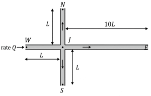
📝 In the pipe network shown in the figure, all pipes have the same cross-section and can be assumed to have the same friction factor. The pipes connecting points W,N and S with point J have an equal length L. The pipe connecting points J and E has a length 10 L. The pressure at the ends N,E and S are equal. The flow rate in the pipe connecting W and J is Q. Assume that the fluid flow is steady, incompressible, and the pressure losses at the pipe entrance and junction are negligible. Consider the following statements:
I. The flow rate in pipe connecting J and E is Q/21.
II. The pressure difference between J and N is equal to the pressure difference between J and E.

Which one of the following options is CORRECT?

(Q) = Flow Rate

(A) I is True and II is False
(B) I is False and II is True
(C) Both I and II are True
(D) Both I and II are False

Solution =

⦾ Flow Network Analysis:
The total flow rate entering at $ W $ is:
$$ Q $$
At junction $ J $, the flow splits towards $ N $, $ S $, and $ E $.

⦾ Head Loss Relationship:
The head loss ($ h_f $) due to friction in a pipe is given by:
$$ h_f \propto f \cdot \frac{L}{D} \cdot \frac{v^2}{2g} $$
Since cross-section and friction factor are equal for all pipes, the head loss is directly proportional to:
$$ h_f \propto L \cdot Q^2 $$

⦾ Considering length:
✓ Pipes $ JN $, $ JS $, and $ JW $ have length $ L $
✓ Pipe $ JE $ has length $ 10L $
Therefore, pipe $ JE $ offers significantly higher resistance compared to the other three.

⦾ Flow Division:
Since the path to $ E $ has 10 times longer length, only a small portion of flow will go towards $ E $. Therefore, the claim in statement I, that flow in $ JE $ is $ Q/21 $, is incorrect without detailed calculation. The actual flow would be very small but not exactly $ Q/21 $.

⦾ Pressure Difference:
At steady state, due to equal pressure at ends $ N $, $ E $, and $ S $, and same flow division symmetry from $ J $, the pressure drop between $ J $ to $ N $ will be equal to the pressure drop from $ J $ to $ E $, as both are determined by frictional resistance from junction $ J $ to the endpoints, though flows differ.
Thus, statement II is correct.

⦾ Final Answer: Option B: I is False and II is True

📝 Consider steady, one-dimensional compressible flow of a gas in a pipe of diameter 1 m. At one location in the pipe, the density and velocity are 1 kg/m³ and 100 m/s, respectively. At a downstream location, the velocity is 170 m/s. If the pressure drop between these two locations is 10 kPa, the force exerted by the gas on the pipe between these two locations is ____ N.

(A) 350π²
(B) 750π
(C) 1000π
(D) 3000

Solution =

⦾ Given:
✓ Diameter (D) = 1 m → Area (A) = π(0.5)² = π/4 m²
✓ Upstream: ρ₁ = 1 kg/m³, V₁ = 100 m/s
✓ Downstream: V₂ = 170 m/s
✓ Pressure drop (P₁ – P₂) = 10 kPa = 10,000 Pa

⦾ Step 1: Apply Continuity Equation
For steady flow, mass flow rate (ṁ) is constant: \[ ṁ = ρ₁AV₁ = ρ₂AV₂ \] \[ 1 \times \frac{π}{4} \times 100 = ρ₂ \times \frac{π}{4} \times 170 \] \[ ρ₂ = \frac{100}{170} = 0.588 \text{ kg/m³} \]
⦾ Step 2: Apply Momentum Equation
Force balance in x-direction: \[ F = ṁ(V₂ – V₁) + (P₂A – P₁A) \] Substitute ṁ = ρ₁AV₁ = 1 × (π/4) × 100 = 25π kg/s: \[ F = 25π(170 – 100) + \left(P₂\frac{π}{4} – P₁\frac{π}{4}\right) \] Given P₁ – P₂ = 10,000 Pa: \[ F = 25π \times 70 – 10,000 \times \frac{π}{4} \] \[ F = 1750π – 2500π = -750π \text{ N} \]
⦾ Step 3: Interpret the Force
The negative sign indicates the force is exerted by the gas on the pipe in the opposite direction. Thus, magnitude is: \[ |F| = 750π \text{ N} \]
⦾ Final Answer: The force exerted by the gas on the pipe is $\boxed{B}$ $750π$ N.

📝 For a steady flow, the velocity field is [ \overrightarrow{v} = (-x^2 + 3y)\hat{i} + (2xy)\hat{j} ] , The magnitude of the acceleration of a particle at (1, -1) is

(A) 2
(B) 1
(C) 2√5
(D) 0

Solution =

Given the velocity field for steady flow: \[ \overrightarrow{v} = (-x^2 + 3y)\hat{i} + (2xy)\hat{j} \]
We need to find the acceleration magnitude at point (1, -1).

⦾ Step 1: Calculate acceleration components
For steady flow, particle acceleration is given by: \[ \overrightarrow{a} = (\overrightarrow{v} \cdot \nabla)\overrightarrow{v} \] Which expands to: \[ a_x = u\frac{\partial u}{\partial x} + v\frac{\partial u}{\partial y} \] \[ a_y = u\frac{\partial v}{\partial x} + v\frac{\partial v}{\partial y} \]
Where: \[ u = -x^2 + 3y, \quad v = 2xy \]
Compute partial derivatives: \[ \frac{\partial u}{\partial x} = -2x, \quad \frac{\partial u}{\partial y} = 3 \] \[ \frac{\partial v}{\partial x} = 2y, \quad \frac{\partial v}{\partial y} = 2x \]
Now calculate acceleration components: \[ a_x = (-x^2 + 3y)(-2x) + (2xy)(3) \] \[ a_y = (-x^2 + 3y)(2y) + (2xy)(2x) \]
⦾ Step 2: Evaluate at point (1, -1)
Substitute x = 1, y = -1: \[ u = -(1)^2 + 3(-1) = -1 -3 = -4 \] \[ v = 2(1)(-1) = -2 \]
Compute acceleration components: \[ a_x = (-4)(-2) + (-2)(3) = 8 – 6 = 2 \] \[ a_y = (-4)(-2) + (-2)(2) = 8 – 4 = 4 \]
⦾ Step 3: Calculate magnitude
Acceleration magnitude: \[ |\overrightarrow{a}| = \sqrt{a_x^2 + a_y^2} = \sqrt{2^2 + 4^2} \]\[= \sqrt{4 + 16} = \sqrt{20} = 2\sqrt{5} \]
⦾ Conclusion:
The correct answer is: \[ \boxed{C\ 2\sqrt{5}} \]

📝 Consider the two-dimensional velocity field given by $\vec{V} = $$ (5 + a_1 x + b_1 y) \hat{i} + (4 + a_2 x + b_2 y) \hat{j}, $ where $ a_1, b_1, a_2, b_2 $ are constants. Which one of the following conditions needs to be satisfied for the flow to be incompressible?

(A) $ a_1 + b_1 = 0 $
(B) $ a_1 + b_2 = 0 $
(C) $ a_2 + b_2 = 0 $
(D) $ a_2 + b_1 = 0 $

Solution =

Given the two-dimensional velocity field: $\vec{V} = $ \[ (5 + a_1 x + b_1 y)\hat{i} + (4 + a_2 x + b_2 y)\hat{j} \] We need to determine the condition for incompressible flow.

⦾ Step 1: Recall incompressibility condition
For incompressible flow in 2D, the divergence of velocity must be zero: \[ \nabla \cdot \vec{v} = \frac{\partial u}{\partial x} + \frac{\partial v}{\partial y} = 0 \] where $ u = 5 + a_1 x + b_1 y $ and $ v = 4 + a_2 x + b_2 y $.

⦾ Step 2: Compute partial derivatives
Calculate the required derivatives: \[ \frac{\partial u}{\partial x} = a_1 \] \[ \frac{\partial v}{\partial y} = b_2 \]
⦾ Step 3: Apply incompressibility condition
Set the divergence to zero: \[ a_1 + b_2 = 0 \]
⦾ Conclusion:
The correct condition is: \[ \boxed{B\ a_1 + b_2 = 0} \]

📝 For a two-dimensional flow, the velocity field is $ \vec{u} = \frac{x}{x^2 + y^2} \hat{i} + \frac{y}{x^2 + y^2} \hat{j}, $ where $ \hat{i} $ and $ \hat{j} $ are the basis vectors in the x-y Cartesian coordinate system. Identify the CORRECT statements from below:

1) The flow is incompressible.
2) The flow is unsteady.
3) y-component of acceleration, $ a_y = \frac{-y}{(x^2 + y^2)^2} $
4) x-component of acceleration, $ a_x = \frac{-(x+y)}{(x^2 + y^2)^2} $

(A) (2) and (3)
(B) (1) and (3)
(C) (1) and (2)
(D) (3) and (4)

Solution =

Given the two-dimensional velocity field: \[ \vec{u} = \frac{x}{x^2 + y^2} \hat{i} + \frac{y}{x^2 + y^2} \hat{j} \] We need to evaluate each statement.

⦾ Step 1: Check incompressibility (Statement 1)
For incompressible flow, ∇·u = 0: \[ \frac{\partial u_x}{\partial x} + \frac{\partial u_y}{\partial y} \]\[= \frac{y^2 – x^2}{(x^2 + y^2)^2} + \frac{x^2 – y^2}{(x^2 + y^2)^2} = 0 \] Statement 1 is TRUE

⦾ Step 2: Check steadiness (Statement 2)
The velocity field has no time dependence → Statement 2 is FALSE

⦾ Step 3: Calculate y-component acceleration (Statement 3)
Using a_y = u·∇u_y: \[ a_y = \frac{x}{x^2+y^2}\frac{\partial u_y}{\partial x} + \frac{y}{x^2+y^2}\frac{\partial u_y}{\partial y} \]\[= \frac{-y}{(x^2 + y^2)^2} \] Statement 3 is TRUE

⦾ Step 4: Calculate x-component acceleration (Statement 4)
Similarly: \[ a_x = \frac{x}{x^2+y^2}\frac{\partial u_x}{\partial x} + \frac{y}{x^2+y^2}\frac{\partial u_x}{\partial y} \]\[= \frac{-x}{(x^2 + y^2)^2} \neq \frac{-(x+y)}{(x^2 + y^2)^2} \] Statement 4 is FALSE

⦾ Conclusion:
Correct statements are (1) and (3): \[ \boxed{B\ (1) \text{ and } (3)} \]

📝 A streamline and an equipotential line in a flow field

(A) Are parallel to each other
(B) Are perpendicular to each other
(C) Intersect at an acute angle
(D) Are identical

Solution =

In fluid mechanics, streamlines represent the direction of fluid flow, while equipotential lines represent locations of equal velocity potential (no change in potential energy).
✓ Streamlines are always tangent to the velocity vector.
✓ Equipotential lines are lines where the velocity potential is constant, and the gradient of velocity potential (which gives the velocity direction) is perpendicular to these lines.
Thus, in irrotational flow fields, streamlines and equipotential lines are always perpendicular at every point.

⦾ Therefore: B) Are perpendicular to each other

📝 Which combination of the following statements about steady incompressible forced vortex flow is correct?

P: Shear stress is zero at all points in the flow.
Q: Vorticity is zero at all points in the flow.
R: Velocity is directly proportional to the radius from the centre of the vortex.
S: Total mechanical energy per unit mass is constant in the entire flow field.

(A) P and Q
(B) R and S
(C) P and R
(D) P and S

Solution =

Forced vortex flow: In forced vortex flow, the fluid rotates like a solid body with constant angular velocity $ \omega $. The tangential velocity is given by:
\[ v_\theta = \omega r \]
This shows that the velocity is directly proportional to the radius from the center.

✓ P: Incorrect. In forced vortex, there is a velocity gradient in the tangential direction ($ \frac{dv_\theta}{dr} \neq 0 $), so shear stress is not zero.
✓ Q: Incorrect. For solid body rotation: \[ \text{Vorticity} = 2\omega \neq 0 \] Therefore, vorticity is not zero.
✓ R: Correct. As shown above, $ v_\theta = \omega r $, hence velocity is directly proportional to radius.
✓ S: Correct. In ideal (non-viscous, incompressible) forced vortex flow, mechanical energy per unit mass remains constant throughout the flow field.

Therefore, the correct combination is: R and S
⦾ Final Answer: Option B

📝 The velocity profile in fully developed laminar flow in a pipe of diameter D is given by ( u(r) = u_0 \left(1 – \frac{4r^2}{D^2}\right) ) where r is the radial distance from the center. If the viscosity of the fluid is μ, the pressure drop across a length L of the pipe is:

(A) $ \frac{\mu u_0 L}{D^2} $
(B) $ \frac{4 \mu u_0 L}{D^2} $
(C) $ \frac{8 \mu u_0 L}{D^2} $
(D) $ \frac{16 \mu u_0 L}{D^2} $

Solution =

The velocity profile in fully developed laminar flow in a pipe of diameter $ D $ is:
\[ u(r) = u_0 \left(1 – \frac{4r^2}{D^2}\right) \]
This is a parabolic profile. We are to find the pressure drop $ \Delta P $ across a length $ L $ of the pipe.

⦾ Step 1: Pressure Drop Formula
For laminar flow, the pressure drop is given by:
\[ \Delta P = \frac{32 \mu U_{\text{avg}} L}{D^2} \]
Where:
✓ $ \mu $: fluid viscosity
✓ $ U_{\text{avg}} $: average velocity
✓ $ L $: pipe length
✓ $ D $: pipe diameter

⦾ Step 2: Calculate Average Velocity
Given the velocity profile:
\[ u(r) = u_0 \left(1 – \frac{4r^2}{D^2} \right) \]
Average velocity is defined as:
\[ U_{\text{avg}} = \frac{2}{R^2} \int_0^R u(r) \cdot r \, dr \]
Let $ R = \frac{D}{2} $. Then:
\[ U_{\text{avg}} = \frac{2 u_0}{R^2} \int_0^R \left( r – \frac{4r^3}{D^2} \right) dr \]
Evaluate the integral:
\[ \int_0^R \left( r – \frac{4r^3}{D^2} \right) dr \]\[= \left[ \frac{r^2}{2} – \frac{r^4}{D^2} \right]_0^R = \frac{R^2}{2} – \frac{R^4}{D^2} \]
Now substitute into the average velocity expression:
\[ U_{\text{avg}} = \frac{2u_0}{R^2} \left( \frac{R^2}{2} – \frac{R^4}{D^2} \right) \]\[= u_0 \left(1 – \frac{2R^2}{D^2} \right) \]
Since $ R = \frac{D}{2} $, we get:
\[ U_{\text{avg}} = u_0 \left(1 – \frac{2(D^2/4)}{D^2} \right) \]\[= u_0 \left(1 – \frac{1}{2} \right) = \frac{u_0}{2} \]
⦾ Step 3: Final Pressure Drop
\[ \Delta P = \frac{32 \mu U_{\text{avg}} L}{D^2} = \frac{32 \mu (u_0 / 2) L}{D^2} \]\[= \frac{16 \mu u_0 L}{D^2} \]
⦾ Final Answer:
\[ \boxed{\Delta P = \frac{16 \mu u_0 L}{D^2}} \]
Correct option: D

📝 A fluid flow is represented by the velocity field $ \vec{V} = ax\hat{i} + ay\hat{j} $ where a is a constant. The equation of streamline passing through a point (1,2) is

(A) $ x – 2y = 0 $
(B) $ 2x + y = 0 $
(C) $ 2x – y = 0 $
(D) $ x + 2y = 0 $

Solution =

Given velocity field:
\[ \vec{V} = ax\,\hat{i} + ay\,\hat{j} \]
The equation for a streamline is:
\[ \frac{dx}{u} = \frac{dy}{v} \]
Substitute $ u = ax $, $ v = ay $:
\[ \frac{dx}{ax} = \frac{dy}{ay} \Rightarrow \frac{dx}{x} = \frac{dy}{y} \]
Integrate both sides:
\[ \int \frac{dx}{x} = \int \frac{dy}{y} \Rightarrow \ln|x| = \ln|y| + C \]\[\Rightarrow \ln\left(\frac{x}{y}\right) = C \]\[\Rightarrow \frac{x}{y} = K \quad \text{(where } K = e^C \text{)} \Rightarrow x = Ky \]
Use the point $ (1, 2) $ to find $ K $:
\[ 1 = K \cdot 2 \Rightarrow K = \frac{1}{2} \Rightarrow x = \frac{1}{2} y \]\[\Rightarrow 2x = y \Rightarrow 2x – y = 0 \]
⦾ Final Answer:
\[ \boxed{2x – y = 0} \] (Correct Option: C)

📝 A static fluid can have

(A) non-zero normal and shear stress
(B) negative normal stress and zero shear stress
(C) positive normal stress and zero shear stress
(D) zero normal stress and non-zero shear stress

Solution =

In a static fluid (i.e., fluid at rest), the stress behavior is governed by basic fluid mechanics principles:

⦾ Key Points:
A fluid at rest cannot resist shear stress — any shear stress will cause it to deform (flow).
→ So, shear stress = 0
The only stress a static fluid can exert is normal stress, and this is simply the fluid pressure acting perpendicular to any surface in contact with the fluid.
Pressure is a positive normal stress (compressive).
→ Hence, non-zero normal stress can exist in the form of positive pressure.

⦾ Therefore:
Normal stress: Present (as pressure), and it’s positive
Shear stress: Always zero in a static fluid

❌ Why other options are incorrect:
✓ A) Non-zero shear stress is not possible in a static fluid.
✓ B) Fluids cannot have negative pressure under normal circumstances, and shear stress must be zero.
✓ D) Zero normal stress is incorrect — fluids always exert pressure.

⦾ Final Answer: C) positive normal stress and zero shear stress

📝 The steady velocity field in an inviscid fluid of density 1.5 is given to be: \[ \vec{V} = (y^2 – x^2)\hat{i} + (2xy)\hat{j} \] Neglecting body forces, the pressure gradient at (x = 1, y = 1) is:

(A) $10\hat{i}$
(B) $20\hat{j}$
(C) $-6\hat{i} – 6\hat{j}$
(D) $-4\hat{i} – 4\hat{j}$

Solution =

Step 1: Understand the Euler Equation
For inviscid flow (μ=0) with negligible body forces, the momentum equation reduces to Euler’s equation:
\[ \rho \frac{D\vec{V}}{Dt} = -\nabla p \] For steady flow, this becomes: \[ \rho (\vec{V} \cdot \nabla) \vec{V} = -\nabla p \]
Step 2: Compute Acceleration Terms
Given $\vec{V} = u\hat{i} + v\hat{j} = (y^2 – x^2)\hat{i} + (2xy)\hat{j}$:
\[ (\vec{V} \cdot \nabla) \vec{V} = u\frac{\partial \vec{V}}{\partial x} + v\frac{\partial \vec{V}}{\partial y} \] Compute partial derivatives:
\[ \frac{\partial \vec{V}}{\partial x} = -2x\hat{i} + 2y\hat{j} \] \[ \frac{\partial \vec{V}}{\partial y} = 2y\hat{i} + 2x\hat{j} \] Now calculate the convective acceleration: \[ (\vec{V} \cdot \nabla) \vec{V} = (y^2 – x^2)(-2x\hat{i} + 2y\hat{j}) \]\[ + (2xy)(2y\hat{i} + 2x\hat{j}) \]
Step 3: Evaluate at (1,1)
At point (1,1): \[ u = 1^2 – 1^2 = 0, \quad v = 2×1×1 = 2 \] \[ \frac{\partial \vec{V}}{\partial x} = -2\hat{i} + 2\hat{j}, \quad \frac{\partial \vec{V}}{\partial y} = 2\hat{i} + 2\hat{j} \] \[ (\vec{V} \cdot \nabla) \vec{V} = 0 + 2(2\hat{i} + 2\hat{j}) = 4\hat{i} + 4\hat{j} \]
Step 4: Calculate Pressure Gradient
From Euler’s equation: \[ \nabla p = -\rho (\vec{V} \cdot \nabla) \vec{V} = -1.5 (4\hat{i} + 4\hat{j}) \]\[ = -6\hat{i} – 6\hat{j} \]
Step 5: Verify Irrotationality
Check if the flow is irrotational (though not necessary for solution):
\[ \omega = \frac{\partial v}{\partial x} – \frac{\partial u}{\partial y} = 2y – (-2y) = 4y \neq 0 \] The flow is rotational at y≠0, so we cannot use Bernoulli’s equation.

Final Answer: $\boxed{C}$

📝 A solid spherical bead of lead (density = 11000 kg/m³) of diameter d = 0.1mm sinks with constant velocity V in a viscous liquid (dynamic viscosity = 1.1 × 10⁻³ kg/m·s). The drag coefficient is CD = 24/Re. Neglect buoyancy. Find the terminal velocity V.

(A) $\frac{1}{24}$ m/s
(B) $\frac{1}{6}$ m/s
(C) $\frac{1}{18}$ m/s
(D) $\frac{1}{12}$ m/s

Solution =

⦾ Given:
✓ Bead diameter (d) = 0.1 mm = 0.0001 m
✓ Lead density (ρ_lead) = 11000 kg/m³
✓ Liquid viscosity (μ) = 1.1 × 10⁻³ kg/m·s
✓ Drag coefficient C_D = 24/Re
✓ Gravity (g) = 10 m/s²

⦾ Solution Steps:
1. Calculate bead weight:
\[ W = \rho_{lead} \cdot \frac{\pi d^3}{6} \cdot g \] \[ W = 11000 \cdot \frac{\pi (0.0001)^3}{6} \cdot 10 \] \[ W \approx 5.76 \times 10^{-8} \, \text{N} \]
2. Drag force expression:
Given formula: \[ D = C_D \cdot \frac{1}{2}\rho V^2 \cdot \frac{\pi d^2}{4} \] With C_D = 24/Re and Re = ρVd/μ: \[ D = \frac{24\mu}{\rho V d} \cdot \frac{1}{2}\rho V^2 \cdot \frac{\pi d^2}{4} \] Simplifies to: \[ D = 3\pi \mu V d \]
3. Force balance at terminal velocity:
\[ W = D \] \[ 5.76 \times 10^{-8} = 3\pi (1.1 \times 10^{-3}) V (0.0001) \] \[ V = \frac{5.76 \times 10^{-8}}{3\pi \times 1.1 \times 10^{-7}} \] \[ V \approx \frac{1}{18} \, \text{m/s} \]
⦾ Final Answer: $\boxed{C}$ $\frac{1}{18}$ m/s

📝 For the stability of a floating body the

(A) centre of buoyancy must coincide with the centre of gravity
(B) centre of buoyancy must be above the centre of gravity
(C) centre of gravity must be above the centre of buoyancy
(D) metacenter must be above the centre of gravity

Solution =

For a floating body to be stable, the metacenter ($ M $) must lie above the center of gravity ($ G $). This ensures a righting moment when the body tilts, restoring equilibrium.

⦾ Key Definitions:
✓ Center of Buoyancy ($ B $): The centroid of the displaced fluid volume.
✓ Center of Gravity ($ G $): The point where the body’s weight acts.
✓ Metacenter ($ M $): The intersection point of the buoyancy line (after tilt) and the original vertical axis.

⦾ Stability Condition:
\[ \text{If } M \text{ is above } G \]\[ \Rightarrow \text{Stable} \\ \text{If } M \text{ coincides with } G \]\[ \Rightarrow \text{Neutral} \\ \text{If } M \text{ is below } G \Rightarrow \text{Unstable} \]
⦾ Why Other Options Are Incorrect:
✓ A) $ B $ need not coincide with $ G $ (neutral stability).
✓ B) $ B $ is usually below $ G $ in stable bodies (e.g., ships).
✓ C) $ G $ can be above $ B $ and still stable if $ M $ is above $ G $.

📝 Consider steady flow of an incompressible fluid through two long and straight pipes of diameters $ d_1 $ and $ d_2 $ arranged in series. Both pipes are of equal length and the flow is turbulent in both pipes. The friction factor for turbulent flow through pipes is of the form: $ f = k (Re)^{-n}$ where ( k ) and ( n ) are known positive constants and ( Re ) is the Reynolds number. Neglecting minor losses, the ratio of the frictional pressure drop in pipe 1 to that in pipe 2, \[ \left( \frac{\Delta P_1}{\Delta P_2} \right), \] is given by:

(A) $ \left( \frac{d_2}{d_1} \right)^{5 – n} $
(B) $ \left( \frac{d_2}{d_1} \right)^5 $
(C) $ \left( \frac{d_2}{d_1} \right)^{3 – n} $
(D) $ \left( \frac{d_2}{d_1} \right)^{5 + n} $

Solution =

We are given two pipes in series with diameters $ d_1 $ and $ d_2 $, equal lengths, and turbulent flow with friction factor $ f = k(Re)^{-n} $, where $ Re $ is the Reynolds number.

⦾ Step 1: Express the pressure drop
The frictional pressure drop in a pipe (Darcy-Weisbach equation) is: \[ \Delta P = f \frac{L}{d} \frac{\rho V^2}{2} \] where:
✓ $ f $ = friction factor
✓ $ L $ = pipe length
✓ $ d $ = pipe diameter
✓ $ \rho $ = fluid density
✓ $ V $ = flow velocity

⦾ Step 2: Relate velocities through continuity
For incompressible flow in series, the volumetric flow rate $ Q $ is constant: \[ Q = V_1 A_1 = V_2 A_2 \]\[ \implies V_1 = V_2 \left(\frac{d_2}{d_1}\right)^2 \]
⦾ Step 3: Express Reynolds number
Reynolds number is: \[ Re = \frac{\rho V d}{\mu} \implies Re \propto V d \] Thus: \[ \frac{Re_1}{Re_2} = \frac{V_1 d_1}{V_2 d_2} = \left(\frac{d_2}{d_1}\right)^2 \cdot \frac{d_1}{d_2} = \frac{d_2}{d_1} \]
⦾ Step 4: Express friction factors
Given $ f = k(Re)^{-n} $, the ratio is: \[ \frac{f_1}{f_2} = \left(\frac{Re_1}{Re_2}\right)^{-n} = \left(\frac{d_2}{d_1}\right)^{-n} \]
⦾ Step 5: Compute pressure drop ratio
Pressure drop ratio: \[ \frac{\Delta P_1}{\Delta P_2} = \frac{f_1 \frac{L}{d_1} \rho V_1^2}{f_2 \frac{L}{d_2} \rho V_2^2} = \frac{f_1}{f_2} \cdot \frac{d_2}{d_1} \cdot \left(\frac{V_1}{V_2}\right)^2 \] Substitute from previous steps: \[ = \left(\frac{d_2}{d_1}\right)^{-n} \cdot \frac{d_2}{d_1} \cdot \left(\frac{d_2}{d_1}\right)^4 = \left(\frac{d_2}{d_1}\right)^{5 – n} \]
⦾ Conclusion:
The correct answer is: \[ \boxed{A\ \left(\frac{d_2}{d_1}\right)^{(5-n)}} \]

📝 The velocity profile inside the boundary layer for flow over a flat plate is given as $ \frac{u}{U_\infty} = \sin\left(\frac{\pi}{2}\frac{y}{\delta}\right) $ where $ U_\infty $ is the free stream velocity and $ \delta $ is the local boundary layer thickness. If $ \delta^* $ is the local displacement thickness, is the local displacement thickness, the value of $ \frac{\delta^*}{\delta} $ is:

(A) $ \frac{2}{\pi} $
(B) $ 1 – \frac{2}{\pi} $
(C) $ 1 + \frac{2}{\pi} $
(D) $ 0 $

Solution =

Given the velocity profile for boundary layer flow over a flat plate: \[ \frac{u}{U_\infty} = \sin\left(\frac{\pi}{2}\frac{y}{\delta}\right) \] where:
✓ $ U_\infty $ = free stream velocity
✓ $ \delta $ = local boundary layer thickness
✓ $ \delta^* $ = displacement thickness to be found

⦾ Step 1: Recall displacement thickness definition
Displacement thickness is defined as: \[ \delta^* = \int_0^\delta \left(1 – \frac{u}{U_\infty}\right) dy \]
⦾ Step 2: Substitute the given velocity profile
Using the given profile: \[ \delta^* = \int_0^\delta \left(1 – \sin\left(\frac{\pi}{2}\frac{y}{\delta}\right)\right) dy \]
⦾ Step 3: Solve the integral
Let $ \eta = \frac{y}{\delta} $, then $ dy = \delta d\eta $, and limits change from 0 to 1: \[ \delta^* = \delta \int_0^1 \left(1 – \sin\left(\frac{\pi}{2}\eta\right)\right) d\eta \] \[ = \delta \left[ \int_0^1 1 \, d\eta – \int_0^1 \sin\left(\frac{\pi}{2}\eta\right) d\eta \right] \] \[ = \delta \left[ 1 – \left( -\frac{2}{\pi} \cos\left(\frac{\pi}{2}\eta\right) \bigg|_0^1 \right) \right] \] \[ = \delta \left[ 1 – \left( -\frac{2}{\pi} (0 – 1) \right) \right] \] \[ = \delta \left[ 1 – \frac{2}{\pi} \right] \]
⦾ Step 4: Compute the ratio
The required ratio is: \[ \frac{\delta^*}{\delta} = 1 – \frac{2}{\pi} \]
⦾ Conclusion: The correct answer is: \[ \boxed{B\ 1 – \frac{2}{\pi}} \]

📝 A smooth pipe of diameter 200 mm carries water. The pressure in the pipe at section S1 (elevation: 10m) is 50kPa. At Section S2 (elevation: 12m) the pressure is 20kPa and velocity is $ 2\, \mathrm{ms}^{-1} $. Density of water is $ 1000\, \mathrm{kgm}^{-3} $ and acceleration due to gravity is $ 9.8\, \mathrm{ms}^{-2} $. Which of the following is TRUE?

(A) flow from S1 to S2 and head loss is 0.53m
(B) flow from S2 to S1 and head loss is 0.53m
(C) flow from S1 to S2 and head loss is 1.06m
(D) flow from S2 to S1 and head loss is 1.06m

Solution =

To solve this, we apply the Bernoulli equation including head loss between two sections $ S_1 $ and $ S_2 $:
\[ \frac{P_1}{\gamma} + \frac{V_1^2}{2g} + z_1 = \frac{P_2}{\gamma} + \frac{V_2^2}{2g} + z_2 + h_f \]
⦾ Where:
✓ $ P_1 = 50\,\text{kPa} = 50000\,\text{Pa} $
✓ $ z_1 = 10\,\text{m} $
✓ $ V_1 = V_2 = 2\,\text{m/s} $ (same diameter, so same velocity)
✓ $ P_2 = 20\,\text{kPa} = 20000\,\text{Pa} $
✓ $ z_2 = 12\,\text{m} $
✓ $ \gamma = \rho g = 1000 \times 9.8 = 9800\,\text{N/m}^3 $

⦾ Step-by-step:
✓ Left side (S1):
\[ \frac{P_1}{\gamma} + \frac{V^2}{2g} + z_1 \]\[ = \frac{50000}{9800} + \frac{2^2}{2 \times 9.8} + 10 \]\[ = 5.102 + 0.204 + 10 = 15.306\,\text{m} \]
✓ Right side (S2):
\[ \frac{P_2}{\gamma} + \frac{V^2}{2g} + z_2 \]\[ = \frac{20000}{9800} + 0.204 + 12 \]\[ = 2.041 + 0.204 + 12 = 14.245\,\text{m} \]
✓ Head loss:
\[ h_f = 15.306 – 14.245 = \boxed{1.06\,\text{m}} \]
✓ Flow direction:
Since total head at $ S_1 > S_2 $, the flow is from $ S_1 $ to $ S_2 $.

⦾ Final Answer:
C. flow from S1 to S2 and head loss is 1.06 m

📝 For a continuity equation given by: $ \nabla \cdot \vec{V} = 0 $ to be valid, where $ \vec{V} $ is the velocity vector, which one of the following is a necessary condition?

(A) steady flow
(B) irrotational flow
(C) inviscid flow
(D) incompressible flow

Solution =

⦾ Correct Answer: D) Incompressible flow

⦾ Explanation:
✓ Steady flow (Option A): No change with respect to time, but density may vary — not sufficient.
✓ Irrotational flow (Option B): Implies zero vorticity ($ \nabla \times \vec{V} = 0 $), not related to mass conservation.
✓ Inviscid flow (Option C): Neglects viscosity, but doesn’t imply anything about compressibility or continuity.
✓ Incompressible flow (Option D): Implies constant density, and the continuity equation becomes: \[ \nabla \cdot \vec{V} = 0 \] which is the condition given in the question.

Thus, the correct and necessary condition for the given continuity equation is incompressible flow.

📝 In a two-dimensional velocity field with velocities u and v along the x and y directions respectively, the convective acceleration along the x-direction is given by

(A) $ u \frac{\partial u}{\partial x} + v \frac{\partial u}{\partial y} $
(B) $ u \frac{\partial u}{\partial x} + v \frac{\partial v}{\partial y} $
(C) $ u \frac{\partial v}{\partial x} + v \frac{\partial u}{\partial y} $
(D) $ v \frac{\partial u}{\partial x} + u \frac{\partial u}{\partial y} $

Solution =

In a two-dimensional velocity field with velocity components $ u $ along the $ x $-direction and $ v $ along the $ y $-direction, the convective acceleration along the x-direction is given by:
\[ a_x = u \frac{\partial u}{\partial x} + v \frac{\partial u}{\partial y} \]
This represents the change in the x-component of velocity due to spatial variations in both $ x $ and $ y $ directions.

⦾ Correct Option: A
\[ \boxed{u \frac{\partial u}{\partial x} + v \frac{\partial u}{\partial y}} \]

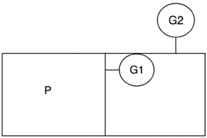
📝 The pressure gauges $ G_1 $ and $ G_2 $ installed on the system show pressures of $ P_{G_1} $ = 5.00 bar and $ P_{G_2} $ =1.00 bar. The value of unknown pressure P is

(A) 1.01 bar
(B) 2.01 bar
(C) 5.00 bar
(D) 7.01 bar

Solution =

⦾ Given:
✓ $ P_{G_1} = 5 \, \text{bar} $
✓ $ P_{G_2} = 1 \, \text{bar} $
✓ $ P_{\text{atm}} = 1.01 \, \text{bar} $

⦾ Step 1: For pressure gauge $ G_2 $
Absolute pressure at $ G_2 $ is calculated as: \[ P_{\text{abs}, G_2} = P_{\text{atm}} + P_{G_2} \]\[ = 1.01 + 1 = 2.01 \, \text{bar} \]
Since this is connected to atmospheric reference, we assume: \[ P_{\text{local atm (for G}_1)} = 2.01 \, \text{bar} \]
⦾ Step 2: For pressure gauge $ G_1 $
Absolute pressure at $ G_1 $ (i.e., pressure $ P $) is: \[ P = P_{\text{local atm}} + P_{G_1} \]\[ = 2.01 + 5 = 7.01 \, \text{bar} \]
⦾ Final Answer: $ \boxed{7.01 \, \text{bar}} $

📝 Match the following non-dimensional numbers with the corresponding definitions:

(A) P-1, Q-3, R-2, S-4
(B) P-3, Q-1, R-2, S-4
(C) P-4, Q-3, R-1, S-2
(D) P-3, Q-1, R-4, S-2

Solution =

(Matching the Non-Dimensional Numbers):
(Symbol => Non-dimensional Number => Matching Definition)
✓ P => Reynolds number => 3
✓ Q => Grashof number => 1
✓ R => Nusselt number => 4
✓ S => Prandtl number => 2

So, the correct matching is:
P → 3
Q → 1
R → 4
S → 2

⦾ Final Answer: Option D

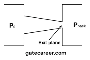
📝 The figure shows a purely convergent nozzle with a steady, inviscid compressible flow of an ideal gas with constant thermophysical properties operating under choked condition. The exit plane shown in the figure is located within the nozzle. If the inlet pressure $ P_0 $ is increased while keeping the back pressure $ P_{\text{back}} $ unchanged, which of the following statements is/are true?

(A) Mass flow rate through the nozzle will remain unchanged.
(B) Mach number at the exit plane of the nozzle will remain unchanged at unity.
(C) Mass flow rate through the nozzle will increase.
(D) Mach number at the exit plane of the nozzle will become more than unity.

Solution =

⦾ Key Concepts:
✓ A convergent nozzle reaches choked flow when the flow at the exit plane reaches Mach number = 1.
✓ Once choked, increasing the upstream total pressure $ P_0 $ while keeping the back pressure $ P_{\text{back}} $ constant does not change the Mach number at the exit; it remains unity.
✓ Mass flow rate through a choked nozzle increases with increase in $ P_0 $, because the mass flow rate under choked conditions is given by:

\[ \dot{m} = C A^\ast P_0 \sqrt{\frac{\gamma}{R T_0}} \left( \frac{2}{\gamma + 1} \right)^{\frac{\gamma + 1}{2(\gamma – 1)}} \]
where $ C $ is a constant, $ A^\ast $ is the throat area. This shows that $ \dot{m} \propto P_0 $, if $ T_0 $ is constant.

⦾ Now consider the options:
A. Mass flow rate through the nozzle will remain unchanged.
→ False, because $ \dot{m} $ increases with $ P_0 $.
B. Mach number at the exit plane of the nozzle will remain unchanged at unity.
→ True, because choked flow ensures $ M = 1 $ at the exit of a convergent nozzle.
C. Mass flow rate through the nozzle will increase.
→ True, from the mass flow rate equation under choked conditions.
D. Mach number at the exit plane of the nozzle will become more than unity.
→ False, since this is not possible in a purely convergent nozzle.

⦾ Correct Answers: B and C

📝 In the following two-dimensional momentum equation for natural convection over a surface immersed in a quiescent fluid at temperature $ T_\infty $ (g is the gravitational acceleration, $ \beta $ is the volumetric thermal expansion coefficient, $ \nu $ is the kinematic viscosity, $ u $ and $ v $ are the velocities in x and y directions, respectively, and $ T $ is the temperature) \[ u \frac{\partial u}{\partial x} + v \frac{\partial u}{\partial y} = g \beta (T – T_\infty) + \nu \frac{\partial^2 u}{\partial y^2}\] The term $ g \beta (T – T_\infty) $ represents.

(A) Ratio of inertial force to viscous force.
(B) Ratio of buoyancy force to viscous force.
(C) Viscous force per unit mass.
(D) Buoyancy force per unit mass.

Solution =

In the 2D momentum equation for natural convection:
\[ u \frac{\partial u}{\partial x} + v \frac{\partial u}{\partial y} = g \beta (T – T_\infty) + \nu \frac{\partial^2 u}{\partial y^2} \]
The term $ g \beta (T – T_\infty) $ represents the buoyancy force per unit mass, which drives natural convection due to density differences caused by temperature gradients.

⦾ Correct Answer: D

📝 For a certain two-dimensional incompressible flow, velocity field is given by $ \vec{u} = 2xy\hat{i} – y^2\hat{j} $ The streamlines for this flow are given by the family of curves

(A) $ x^2 y^2 = \text{constant} $
(B) $ x y^2 = \text{constant} $
(C) $ 2xy – y^2 = \text{constant} $
(D) $ xy = \text{constant} $

Solution =

Given the two-dimensional incompressible flow velocity field: \[ \vec{u} = 2xy\hat{i} – y^2\hat{j} \] We need to find the equation for its streamlines.

⦾ Step 1: Recall streamline equation
For 2D flow, streamlines satisfy: \[ \frac{dy}{dx} = \frac{v}{u} = \frac{-y^2}{2xy} = \frac{-y}{2x} \]
⦾ Step 2: Solve the differential equation
Separate variables: \[ \frac{dy}{y} = \frac{-dx}{2x} \] Integrate both sides: \[ \ln|y| = -\frac{1}{2}\ln|x| + C \] Exponentiate: \[ y = e^C x^{-1/2} \implies y\sqrt{x} = \text{constant} \] Square both sides: \[ x y^2 = \text{constant} \]
⦾ Step 3: Verify with given options
The solution matches option B: $ xy^2 = \text{constant} $

⦾ Conclusion:
The correct answer is: \[ \boxed{B\ xy^2 = \text{constant}} \]

📝 Assuming constant temperature condition and air to be an ideal gas, the variation in atmospheric pressure with height calculated from fluid statics is

(A) linear
(B) exponential
(C) quadratic
(D) cubic

Solution =

To determine how atmospheric pressure varies with height under constant temperature conditions for an ideal gas, we analyze the hydrostatic equilibrium and ideal gas law.

⦾ Step 1: Hydrostatic Equilibrium
The pressure variation with height is given by: \[ \frac{dP}{dz} = -\rho g \] where:
✓ $ P $ = pressure
✓ $ \rho $ = density
✓ $ g $ = acceleration due to gravity
✓ $ z $ = height

⦾ Step 2: Ideal Gas Law
For an ideal gas at constant temperature: \[ P = \rho R T \] where:
✓ $ R $ = specific gas constant
✓ $ T $ = temperature (constant)
Thus, density can be expressed as: \[ \rho = \frac{P}{RT} \]
⦾ Step 3: Differential Equation
Substitute the density into the hydrostatic equation: \[ \frac{dP}{dz} = -\left(\frac{P}{RT}\right) g \] Rearrange: \[ \frac{dP}{P} = -\frac{g}{RT} dz \]
⦾ Step 4: Solve the Differential Equation
Integrate both sides: \[ \int \frac{dP}{P} = -\frac{g}{RT} \int dz \] \[ \ln P = -\frac{g}{RT} z + C \] Exponentiate to solve for pressure: \[ P = P_0 e^{-\frac{g}{RT}z} \] where $ P_0 $ is the pressure at $ z = 0 $.

⦾ Step 5: Conclusion
The pressure varies exponentially with height under constant temperature conditions.

⦾ Final Answer:
The correct answer is: \[ \boxed{B\ \text{exponential}} \]

📝 The volumetric flow rate (per unit depth) between two streamlines having stream functions Ψ₁ and Ψ₂ is

(A) |Ψ₁ + Ψ₂|
(B) Ψ₁Ψ₂
(C) Ψ₁/Ψ₂
(D) |Ψ₁ – Ψ₂|

Solution =

The volumetric flow rate (per unit depth) between two streamlines is determined by the difference in their stream function values.

⦾ Key Concept:
In fluid mechanics, the stream function (Ψ) has these properties:
✓ The flow rate between two streamlines is equal to the difference in their stream function values
✓ This relationship holds for both 2D incompressible flow and axisymmetric flow
✓ The direction of flow is from the higher Ψ value to the lower Ψ value

⦾ Mathematical Representation:
The volumetric flow rate per unit depth between two streamlines is: \[ Q = |Ψ_1 – Ψ_2| \] where:
✓ $ Ψ_1 $ = stream function value of first streamline
✓ $ Ψ_2 $ = stream function value of second streamline

⦾ Analysis of Options:
A. |Ψ₁ + Ψ₂| – Incorrect (sum is not physically meaningful here)
B. Ψ₁Ψ₂ – Incorrect (product of stream functions has no flow interpretation)
C. Ψ₁/Ψ₂ – Incorrect (ratio of stream functions is not relevant)
D. |Ψ₁ – Ψ₂| – Correct (matches the fundamental definition)

⦾ Conclusion:
The correct answer is: \[ \boxed{D\ |Ψ_1 – Ψ_2|} \]

📝 A hydraulic turbine develops 1000kW power for a head of 40m. If the head is reduced to 20m, the power developed (in kW) is

(A) 177
(B) 354
(C) 500
(D) 707

Solution =

To solve this, we use the affinity laws for hydraulic turbines, specifically the relationship between power and head:
\[ P \propto H^{3/2} \]
⦾ Given:
✓ $ P_1 = 1000 \, \text{kW} $
✓ $ H_1 = 40 \, \text{m} $
✓ $ H_2 = 20 \, \text{m} $

⦾ Using the relationship:
\[ \frac{P_2}{P_1} = \left( \frac{H_2}{H_1} \right)^{3/2} = \left( \frac{20}{40} \right)^{3/2} \]\[= \left( \frac{1}{2} \right)^{3/2} = \frac{1}{2^{3/2}} = \frac{1}{\sqrt{8}} \approx 0.3536 \]
So the power developed at 20 m head is:
\[ P_2 = P_1 \times 0.3536 = 1000 \times 0.3536 \]\[\approx 354 \, \text{kW} \]
⦾ Final Answer: $\boxed{\text{B. 354}}$

📝 Which combination of the following statements is correct?

P. A gas cools upon expansion only when its Joule-Thomson co-efficient is positive in the temperature range of expansion.
Q. For a system undergoing a process, its entropy remains constant only when the process is reversible.
R. The work done by a closed system in an adiabatic process is a point function.
S. A liquid expands upon freezing when the slope of its fusion curve on Pressure-Temperature diagram is negative.

(A) R and S
(B) P and Q
(C) Q, R and S
(D) P, Q and R

Solution =

⦾ Statement P:
A gas cools upon expansion only when its Joule-Thomson coefficient is positive in the temperature range of expansion.
✓ The Joule-Thomson coefficient ($ \mu_{JT} $) determines whether a gas cools or heats upon expansion (throttling process).
✓ If $ \mu_{JT} > 0 $, the gas cools upon expansion.
✓ If $ \mu_{JT} < 0 $, the gas heats upon expansion.
Correctness: True because cooling occurs only when $ \mu_{JT} > 0 $.

⦾ Statement Q:
For a system undergoing a process, its entropy remains constant only when the process is reversible.
✓ Entropy ($ S $) remains constant ($ \Delta S = 0 $) for reversible adiabatic processes.
✓ However, entropy can also remain constant in other isentropic processes (not necessarily reversible if there is compensating irreversibility).
Correctness: False because entropy can remain constant even in some irreversible processes.

⦾ Statement R:
The work done by a closed system in an adiabatic process is a point function.
✓ In an adiabatic process, no heat is transferred ($ Q = 0 $). From the First Law: \[ \Delta U = -W \]
✓ Since $ \Delta U $ (change in internal energy) is a point function (depends only on initial and final states), $ W $ is also a point function.
Correctness: True.

⦾ Statement S:
A liquid expands upon freezing when the slope of its fusion curve on the Pressure-Temperature diagram is negative.
✓ The fusion curve (solid-liquid equilibrium) on a $ P-T $ diagram has a slope given by the Clausius-Clapeyron equation: \[ \frac{dP}{dT} = \frac{\Delta S}{\Delta V} \]
✓ If the slope is negative, $ \Delta V $ (volume change upon freezing) must be negative (i.e., the liquid expands upon freezing, as in water).
Correctness: True.

⦾ Combination Analysis:
P: True
Q: False
R: True
S: True

The correct combination is R and S (Option A).

⦾ Note: Option C (Q, R, and S) is incorrect because Q is false. Option D (P, Q, and R) is incorrect because Q is false. Option B (P and Q) is incorrect because Q is false.

📝 A leaf is caught in a whirlpool. At a given instant, the leaf is at a distance of 120 m from the center of the whirlpool. The whirlpool can be described by the following velocity distribution: $ V_r = -\left( \frac{60 \times 10^3}{2 \pi r} \right) \, \text{m/s} $ and $ V_\theta = \frac{300 \times 10^3}{2 \pi r} \, \text{m/s} $, where $ r $ (in meters) is the distance from the center of the whirlpool. What will be the distance of the leaf from the center when it has moved through half a revolution?

(A) 48 m
(B) 64 m
(C) 120 m
(D) 142 m

Solution =

A leaf is caught in a whirlpool. At a given instant, the leaf is at a distance of 120 m from the center of the whirlpool. The velocity distribution is given by:
$ V_r = -\left( \frac{60 \times 10^3}{2\pi r} \right) \, \text{m/s}, $$ V_\theta = \frac{300 \times 10^3}{2\pi r} \, \text{m/s} $
We are to find the distance from the center after the leaf has moved through half a revolution, i.e., $ \theta = \pi $ radians.

⦾ Step-by-step Solution:
Angular velocity: \[ \frac{d\theta}{dt} = \frac{V_\theta}{r} = \frac{300 \times 10^3}{2\pi r^2} \]
Radial velocity: \[ \frac{dr}{dt} = V_r = -\frac{60 \times 10^3}{2\pi r} \]
Divide both expressions to eliminate time $ t $: \[ \frac{dr}{d\theta} = \frac{\frac{dr}{dt}}{\frac{d\theta}{dt}} = \frac{-\frac{60 \times 10^3}{2\pi r}}{\frac{300 \times 10^3}{2\pi r^2}} \]\[ = -\frac{60 \times 10^3}{300 \times 10^3} \cdot r = -\frac{1}{5}r \]
This is a separable differential equation: \[ \frac{dr}{r} = -\frac{1}{5} d\theta \]
Integrate both sides: \[ \int_{r_0}^{r} \frac{1}{r} dr = -\frac{1}{5} \int_0^{\pi} d\theta \] \[ \ln r – \ln r_0 = -\frac{\pi}{5} \Rightarrow \ln\left(\frac{r}{r_0}\right) \] \[= -\frac{\pi}{5} \Rightarrow \frac{r}{r_0} = e^{-\pi/5} \Rightarrow r = r_0 \cdot e^{-\pi/5} \]
Given $ r_0 = 120 \, \text{m} $, we get: \[ r = 120 \cdot e^{-\pi/5} \approx 120 \cdot e^{-0.6283} \]\[\approx 120 \cdot 0.533 \approx 63.96 \, \text{m} \]
⦾ Final Answer:
\[ \boxed{64 \, \text{m}} \quad \text{(Option B)} \]

📝 A centrifugal pump is required to pump water to an open water tank situated 4 km away from the location of the pump through a pipe of diameter 0.2 m having Darcy’s friction factor of 0.01. The average speed of water in the pipe is 2 m/s. If it is maintain a constant head of 5 m in the tank, neglecting other minor losses, the absolute discharge pressure at the pump exit is

(A) 0.449 bar
(B) 5.503 bar
(C) 44.911 bar
(D) 55.203 bar

Solution =

⦾ Given:
✓ Distance from pump to tank: $ L = 4\, \text{km} = 4000\, \text{m} $
✓ Pipe diameter: $ D = 0.2\, \text{m} $
✓ Darcy’s friction factor: $ f = 0.01 $
✓ Water velocity in pipe: $ v = 2\, \text{m/s} $
✓ Head to be maintained in tank: $ H_{\text{tank}} = 5\, \text{m} $
✓ Atmospheric pressure: $ P_{\text{atm}} = 1.01\, \text{bar} $
✓ Minor losses: Neglected

⦾ Step 1: Friction head loss (Darcy-Weisbach equation)
\[ h_f = f \cdot \frac{L}{D} \cdot \frac{v^2}{2g} \] Substituting the values: \[ h_f = 0.01 \cdot \frac{4000}{0.2} \cdot \frac{2^2}{2 \cdot 9.81} \] \[ h_f = 0.01 \cdot 20000 \cdot \frac{4}{19.62} \] \[= 200 \cdot 0.2039 = 40.78\, \text{m} \]
⦾ Step 2: Total head required at pump discharge
\[ H_{\text{pump}} = h_f + H_{\text{tank}} \] \[= 40.78 + 5 = 45.78\, \text{m} \]
⦾ Step 3: Convert head to pressure
\[ P = \rho g H \] where $ \rho = 1000\, \text{kg/m}^3 $, $ g = 9.81\, \text{m/s}^2 $ \[ P = 1000 \cdot 9.81 \cdot 45.78 = 449114.1\, \text{Pa} \] Converting to bar: \[ P = \frac{449114.1}{100000} \] \[= \boxed{4.491\, \text{bar (gauge pressure)}} \]
⦾ Step 4: Add atmospheric pressure for absolute pressure
\[ P_{\text{abs}} = 4.491 + 1.01 = \boxed{5.501\, \text{bar}} \]
⦾ Final Answer: Option B: 5.503 bar

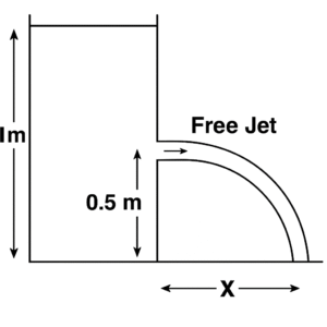
📝 A tank open at the top with a water level of 1 m, as shown in the figure, has a hole at a height of 0.5 m. A free jet leaves horizontally from the smooth hole. The distance X (in m) where the jet strikes the floor is

(A) 0.5
(B) 1
(C) 2
(D) 4

Solution =

⦾ Given:
✓ Height of water level from hole: $ h = 0.5 \, \text{m} $
✓ Height of hole from ground: $ s = 0.5 \, \text{m} $

⦾ Step 1: Velocity of water jet from the hole (Torricelli’s theorem)
\[ v = \sqrt{2gh} \]
⦾ Step 2: Time taken to fall a vertical distance $ s $
Using second equation of motion for free fall:
\[ t = \sqrt{\frac{2s}{g}} \]
⦾ Step 3: Horizontal distance traveled
\[ X = v \cdot t = \sqrt{2gh} \cdot \sqrt{\frac{2s}{g}} = \sqrt{4hs} \]
Substitute $ h = 0.5 \, \text{m}, s = 0.5 \, \text{m} $:
\[ X = \sqrt{4 \cdot 0.5 \cdot 0.5} = \sqrt{1} = 1 \, \text{m} \]
⦾ Final Answer:
\[ \boxed{1 \, \text{m}} \quad \text{(Option B)} \]

📝 A two dimensional flow has velocities in $ x $ and $ y $ directions given by $ u = 2xyt $ and $ v = -y^2 t $, where ( t ) denotes time. The equation for streamline passing through ( x = 1, y = 1 ) is:

(A) $ x^2 y = 1 $
(B) $ x y^2 = 1 $
(C) $ x^2 y^2 = 1 $
(D) $ \frac{x}{y^2} = 1 $

Solution =

A two-dimensional flow has velocities in x and y directions given by $ u = 2xyt $ and $ v = -y^2 t $, where $ t $ denotes time. The equation for the streamline passing through $ x = 1, y = 1 $ is:

⦾ Streamline Equation:
The differential equation for streamlines is: \[ \frac{dy}{dx} = \frac{v}{u} \]
Substitute the given values of $ u $ and $ v $: \[ \frac{dy}{dx} = \frac{-y^2 t}{2xyt} = \frac{-y}{2x} \] The time $ t $ cancels out, so the streamline shape is time-independent (though the pathline would be time-dependent).
Now solve: \[ \frac{dy}{dx} = \frac{-y}{2x} \Rightarrow \frac{dy}{y} = \frac{-dx}{2x} \]
Integrate both sides: \[ \int \frac{1}{y} \, dy = -\frac{1}{2} \int \frac{1}{x} \, dx \Rightarrow \ln y \] \[= -\frac{1}{2} \ln x + C \] \[ \ln y + \frac{1}{2} \ln x = C \Rightarrow \ln(y x^{1/2}) = C \] \[\Rightarrow y x^{1/2} = C_1 \Rightarrow x^{1/2} y = C_1 \] \[\Rightarrow \boxed{x y^2 = \text{constant}} \]
Apply the condition $ x = 1, y = 1 $: \[ 1 \cdot 1^2 = 1 \Rightarrow \text{constant} = 1 \]

⦾ Final Streamline Equation:
\[ \boxed{x y^2 = 1} \]

⦾ Correct Answer: Option B

📝 For a two-dimensional, incompressible flow having velocity components u and v in the x and y directions, respectively, the expression $$ \frac{\partial (u^2)}{\partial x} + \frac{\partial (uv)}{\partial y} $$ can be simplified to:

(A) $ u \frac{\partial u}{\partial x} + u \frac{\partial v}{\partial y} $
(B) $ 2u \frac{\partial u}{\partial x} + u \frac{\partial v}{\partial y} $
(C) $ 2u \frac{\partial u}{\partial x} + v \frac{\partial u}{\partial y} + u \frac{\partial v}{\partial y} $
(D) $ v \frac{\partial u}{\partial x} + v \frac{\partial v}{\partial y} $

Solution =

⦾ Step-by-step Simplification: We are given the expression for a two-dimensional incompressible flow with velocity components $ u $ and $ v $ in the $ x $ and $ y $ directions respectively:
\[ \frac{\partial (u^2)}{\partial x} + \frac{\partial (uv)}{\partial y} \]
We aim to simplify this expression.

⦾ Step 1: Apply the product rule
\[ \frac{\partial (u^2)}{\partial x} = 2u \frac{\partial u}{\partial x} \]
\[ \frac{\partial (uv)}{\partial y} = u \frac{\partial v}{\partial y} + v \frac{\partial u}{\partial y} \]
⦾ Step 2: Combine the terms
\[ \frac{\partial (u^2)}{\partial x} + \frac{\partial (uv)}{\partial y} \] \[= 2u \frac{\partial u}{\partial x} + u \frac{\partial v}{\partial y} + v \frac{\partial u}{\partial y} \]
⦾ Step 3: Group the terms neatly
\[ = 2u \frac{\partial u}{\partial x} + v \frac{\partial u}{\partial y} + u \frac{\partial v}{\partial y} \]
⦾ Final Answer: Option C
\[ \boxed{ 2u \frac{\partial u}{\partial x} + v \frac{\partial u}{\partial y} + u \frac{\partial v}{\partial y} } \]

📝 For a floating body, buoyant force acts at the

(A) centroid of the floating body
(B) center of gravity of the body
(C) centroid of the fluid vertically below the body
(D) centroid of the displaced fluid

Solution =

For a floating body, the buoyant force and its point of application are determined by Archimedes’ principle:

⦾ Key Concept:
The buoyant force:
✓ Equals the weight of the displaced fluid
✓ Acts vertically upward
Passes through the centroid of the displaced fluid volume (called the center of buoyancy)

⦾ Analysis of Options:
A. centroid of the floating body – Incorrect (not relevant for buoyancy)
B. center of gravity of the body – Incorrect (this is where weight acts)
C. centroid of the fluid vertically below the body – Incorrect (misinterpretation)
D. centroid of the displaced fluid – Correct (this is the center of buoyancy)

⦾ Visualization:
The buoyant force acts through the center of buoyancy (B), while the weight acts through the center of gravity (G). The relative positions of B and G determine stability.

⦾ Conclusion:
The correct answer is: \[ \boxed{D\ \text{centroid of the displaced fluid}} \]

📝 The instantaneous stream-wise velocity of a turbulent flow is given as follows: \[ u(x, y, z, t) = \bar{u}(x, y, z) + u'(x, y, z, t) \] The time-average of the fluctuating velocity ( u'(x, y, z, t) ) is:

(A) $ \frac{u’}{2} $
(B) $ -\frac{\bar{u}}{2} $
(C) zero
(D) $ \frac{\bar{u}}{2} $

Solution =

Given the instantaneous stream-wise velocity in turbulent flow: \[ u(x, y, z, t) = \tilde{u}(x, y, z) + u'(x, y, z, t) \] where:
✓ $\tilde{u}$ = time-averaged velocity component
✓ $u’$ = fluctuating velocity component

⦾ Key Concept:
In Reynolds decomposition for turbulent flow:
The time-average of the steady component $\tilde{u}$ is $\tilde{u}$ itself
The time-average of the fluctuating component $u’$ is zero by definition
Mathematically: \[ \overline{u’} = \lim_{T\to\infty} \frac{1}{T} \int_0^T u’ \, dt = 0 \]

⦾ Analysis of Options:
A. $u’/2$ – Incorrect (fluctuations average to zero, not half their value)
B. $-\tilde{u}/2$ – Incorrect (no relation between mean and fluctuation averages)
C. zero – Correct (by definition of Reynolds decomposition)
D. $\tilde{u}/2$ – Incorrect (mean component doesn’t affect fluctuation average)

⦾ Physical Interpretation:
The fluctuating component $u’$ represents random deviations from the mean, which:
✓ Have positive and negative values with equal probability over time
✓ Cancel out when averaged over sufficiently long time periods

⦾ Conclusion:
The correct answer is: \[ \boxed{C\ \text{zero}} \]

📝 Which of the following statements are TRUE, when the cavitation parameter σ=0 ?
(i) the local pressure is reduced to vapor pressure
(ii) cavitation starts
(iii) boiling of liquid starts
(iv) cavitation stops

(A) (i), (ii) and (iv)
(B) only (ii) and (iii)
(C) (i), (iii) and (iv)
(D) (i), (ii) and (iii)

Solution =

The cavitation parameter (also called Thoma cavitation number, denoted by $ \sigma $) is given by:
\[ \sigma = \frac{P_{\text{atm}} – P_v}{\frac{1}{2} \rho V^2} \]
⦾ Where:
✓ $ P_{\text{atm}} $ = local atmospheric or reference pressure
✓ $ P_v $ = vapor pressure of the liquid
✓ $ \rho $ = density
✓ $ V $ = characteristic velocity of flow
✓ When $ \sigma = 0 $:
\[ P_{\text{atm}} = P_v \]
This implies the local pressure is equal to vapor pressure.

⦾ Now evaluate each statement:
(i) The local pressure is reduced to vapor pressure
True — by definition of $ \sigma = 0 $
(ii) Cavitation starts
True — cavitation starts when local pressure drops to or below vapor pressure
(iii) Boiling of liquid starts
True — if local pressure = vapor pressure, boiling can occur, especially in high-velocity regions
(iv) Cavitation stops
False — cavitation starts when local pressure drops to vapor pressure; it doesn’t stop.

⦾ Correct Answer: D) (i), (ii) and (iii)

📝 A phenomenon is modeled using n dimensional variables with k primary dimensions. The number of non-dimensional variables is

(A) k
(B) n
(C) n-k
(D) n+k

Solution =

This question is based on the Buckingham π-theorem, a key concept in dimensional analysis.

⦾ Buckingham π-theorem states:
If a physical phenomenon is described by $ n $ dimensional variables and these involve $ k $ fundamental (primary) dimensions (like Mass, Length, Time), then:
Number of independent non-dimensional groups (π terms) = n – k

⦾ Final Answer:
\[ \boxed{\text{C. } n – k} \]

📝 A model of a hydraulic turbine is tested at a head of 1/4th of that under which the full scale turbine works. The diameter of the model is half of that of the full scale turbine. If N is the RPM of the full scale turbine, then the RPM of the model will be

(A) N/4
(B) N/2
(C) N
(D) 2N

Solution =

To solve this problem, we will use the principle of dynamic similarity for hydraulic turbines. This principle states that for a model and a prototype to have similar flow conditions, their dimensionless parameters must be equal. In this case, we’ll use the head coefficient.

⦾ Given Values:
✓ Head of the model: $H_m = \frac{1}{4}H_f$
✓ Diameter of the model: $D_m = \frac{1}{2}D_f$
✓ RPM of the full-scale turbine: $N_f = N$
Our goal is to find the RPM of the model, $N_m$.

⦾ The Head Coefficient:
The head coefficient, a key dimensionless parameter, must be the same for both the model and the full-scale turbine.
\[ C_H = \frac{gH}{N^2D^2} \]
Setting the head coefficients equal for the model ($m$) and the full-scale turbine ($f$):
\[ \frac{gH_m}{N_m^2D_m^2} = \frac{gH_f}{N_f^2D_f^2} \]
We can cancel out the constant $g$ from both sides:
\[ \frac{H_m}{N_m^2D_m^2} = \frac{H_f}{N_f^2D_f^2} \]
⦾ Substitution and Final Result:
Now, let’s substitute the given relationships into the equation:
\[ \frac{\frac{1}{4}H_f}{N_m^2 (\frac{1}{2}D_f)^2} = \frac{H_f}{N^2D_f^2} \] \[ \frac{\frac{1}{4}H_f}{N_m^2 \frac{1}{4}D_f^2} = \frac{H_f}{N^2D_f^2} \] \[ \frac{H_f}{N_m^2D_f^2} = \frac{H_f}{N^2D_f^2} \]
By comparing both sides of the equation, it is clear that:
$ N_m^2 = N^2 $ \[ N_m = N \]

⦾ Conclusion
The rotational speed (RPM) of the model turbine is equal to the rotational speed of the full-scale turbine.

The correct option is C.

📝 A smooth flat plate with a sharp leading edge is placed along a gas stream flowing at U = 10 m/s. The thickness of the boundary layer at section r-s is 10 mm, the breadth of the plate is 1 m (into the paper) and the density of the gas $ \rho = 1.0 \, \text{kg/m}^3 $. Assume that the boundary layer is thin, two-dimensional, and follows a linear velocity distribution, $ u(y) = U \left( \frac{y}{\delta} \right) $, the section r-s, where y is the height from plate.
The mass flow rate (in kg/s) across the section q-r is:

(A) zero
(B) 0.05
(C) 0.1
(D) 0.15

Solution =

⦾ Given:
✓ Free-stream velocity, $ U = 10 \, \text{m/s} $
✓ Boundary layer thickness, $ \delta = 10 \, \text{mm} = 0.01 \, \text{m} $
✓ Plate breadth, $ b = 1 \, \text{m} $
✓ Gas density, $ \rho = 1.0 \, \text{kg/m}^3 $
✓ Linear velocity profile: $ u(y) = U \left( \frac{y}{\delta} \right) $
Objective: Calculate the mass flow rate (in kg/s) across section $ q-r $.

⦾ Step 1: Understand the flow scenario
The free-stream flow (outside boundary layer) has uniform velocity $ U $. Inside the boundary layer ($ 0 \leq y \leq \delta $), the velocity follows:
\[ u(y) = U \left( \frac{y}{\delta} \right) \] ⦾ Step 2: Compute mass flow rate in boundary layer
Mass flow rate per unit width within boundary layer:
\[ \dot{m}_{\text{boundary}} = \rho \int_{0}^{\delta} u(y) \, dy \] \[= \rho \int_{0}^{\delta} U \left( \frac{y}{\delta} \right) dy \] \[ = \rho U \int_{0}^{\delta} \frac{y}{\delta} \, dy = \rho U \left[ \frac{y^2}{2\delta} \right]_{0}^{\delta} \] \[ = \rho U \left( \frac{\delta^2}{2\delta} – 0 \right) = \rho U \frac{\delta}{2} \] ⦾ Step 3: Plug in given values
\[ \dot{m}_{\text{boundary}} = (1.0 \, \text{kg/m}^3) \times (10 \, \text{m/s}) \] \[\times \left( \frac{0.01 \, \text{m}}{2} \right) = 0.05 \, \text{kg/s} \] ⦾ Step 4: Account for plate width
Since plate breadth $ b = 1 \, \text{m} $:
\[ \dot{m} = \dot{m}_{\text{boundary}} \times b = 0.05 \, \text{kg/s} \times 1 \] \[= 0.05 \, \text{kg/s} \] ⦾ Step 5: Compare with free-stream flow
For reference, free-stream mass flow rate would be:
\[ \dot{m}_{\text{free}} = \rho U \delta = 1.0 \times 10 \times 0.01 \] \[= 0.1 \, \text{kg/s} \] The boundary layer reduces this by half due to slower velocities near the plate.

⦾ Final Answer: The mass flow rate across section $ q-r $ is 0.05 kg/s, corresponding to option B.

📝 An incompressible fluid (kinematic viscosity, $7.4 \times 10^{-7} \, \text{m}^2/\text{s}$, specific gravity, 0.88) is held between two parallel plates. If the top late is moved with a velocity of 0.5 m/s while the bottom one is held stationary, the fluid attains a linear velocity profile in the gap of 0.5 mm between these plates; the shear stress in Pascals on the surface of top plate is

(A) $ 0.651 \times 10^{-3} $
(B) $ 0.651 $
(C) $ 6.51 $
(D) $ 0.651 \times 10^{3} $

Solution =

⦾ Given:
✓ Kinematic viscosity ($\nu$): $7.4 \times 10^{-7} \, \text{m}^2/\text{s}$
✓ Specific gravity (SG): 0.88
✓ Velocity of top plate ($U$): 0.5 m/s
✓ Gap between plates ($h$): 0.5 mm = $0.5 \times 10^{-3} \, \text{m}$
✓ Velocity profile: Linear (simple shear flow)

⦾ Solution:
1. Calculate the dynamic viscosity ($\mu$):
The specific gravity is the ratio of the fluid’s density to water’s density ($\rho_{\text{water}} = 1000 \, \text{kg/m}^3$):
\[ \rho = \text{SG} \times \rho_{\text{water}} = 0.88 \times 1000 \] \[= 880 \, \text{kg/m}^3 \] The dynamic viscosity is:
\[ \mu = \nu \times \rho = 7.4 \times 10^{-7} \times 880 \] \[= 6.512 \times 10^{-4} \, \text{Pa·s} \] 2. Determine the shear rate ($\frac{du}{dy}$):
For a linear velocity profile:
\[ \frac{du}{dy} = \frac{U}{h} = \frac{0.5}{0.5 \times 10^{-3}} = 1000 \, \text{s}^{-1} \] 3. Calculate the shear stress ($\tau$):
Using Newton’s law of viscosity:
\[ \tau = \mu \frac{du}{dy} = 6.512 \times 10^{-4} \times 1000 \] \[= 0.6512 \, \text{Pa} \] ⦾ Final Answer:
The shear stress on the surface of the top plate is approximately $0.651 \, \text{Pa}$, which corresponds to option B.

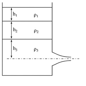
📝 A large tank with a nozzle attached contains three immiscible, inviscid fluids as shown. Assuming that the changes in h1, h2 and h3 are negligible, the instantaneous discharge velocity is

(A) $\sqrt{2gh_3 \left( 1 + \frac{\rho_1}{\rho_3} \frac{h_1}{h_3} + \frac{\rho_2}{\rho_3} \frac{h_2}{h_3} \right)}$
(B) $\sqrt{2g(h_1 + h_2 + h_3)}$
(C) $\sqrt{2g \left( \frac{\rho_1 h_1 + \rho_2 h_2 + \rho_3 h_3}{\rho_1 + \rho_2 + \rho_3} \right)}$
(D) $\sqrt{2g \left( \frac{\rho_1 h_2 h_3 + \rho_2 h_3 h_1 + \rho_3 h_1 h_2}{\rho_1 h_1 + \rho_2 h_2 + \rho_3 h_3} \right)}$

Solution =

To find the instantaneous discharge velocity from the nozzle, we use Bernoulli’s equation and the concept of pressure at the nozzle due to the static fluid column made up of three immiscible, inviscid fluids.

⦾ Given:
✓ Fluid layers: $ \rho_1, h_1 $, $ \rho_2, h_2 $, $ \rho_3, h_3 $
✓ Pressure at nozzle exit is atmospheric.
✓ Changes in $ h_1, h_2, h_3 $ are negligible.
Apply Bernoulli’s equation between the free surface and the nozzle exit.

⦾ Pressure at the nozzle (just before exit):
The pressure at the bottom (nozzle level) is the sum of hydrostatic pressures of all three fluids above it:
\[ P = \rho_1 g h_1 + \rho_2 g h_2 + \rho_3 g h_3 \]
At the nozzle exit, pressure is atmospheric, and velocity is $ V $. Applying Bernoulli’s theorem:
\[ \rho_1 g h_1 + \rho_2 g h_2 + \rho_3 g h_3 = \frac{1}{2} \rho_3 V^2 \]

⦾ Solving for $ V $:
\[ V = \sqrt{ \frac{2}{\rho_3} \left( \rho_1 g h_1 + \rho_2 g h_2 + \rho_3 g h_3 \right) } \] \[ V = \sqrt{ 2g \left( h_3 + \frac{\rho_1}{\rho_3} h_1 + \frac{\rho_2}{\rho_3} h_2 \right) } \]

⦾ Correct Option:
\[ \boxed{ \sqrt{2gh_3 \left( 1 + \frac{\rho_1}{\rho_3} \frac{h_1}{h_3} + \frac{\rho_2}{\rho_3} \frac{h_2}{h_3} \right)} } \] \[\text{(Option A)} \]

📝 The velocity field of an incompressible flow in a Cartesian system is represented by

(A) $-4xz + 6xy$
(B) $-4xy – 4xz$
(C) $4xz – 6xy$
(D) $4xy + 4xz$

Solution =

To determine the correct expression for $ v $ in the given velocity field, we’ll use the incompressibility condition for the flow, which requires that the divergence of the velocity field is zero:
\[ \nabla \cdot \vec{V} = 0 \] Given the velocity field:
\[ \vec{V} = u\hat{i} + v\hat{j} + w\hat{k} \]\[= 2(x^2 – y^2)\hat{i} + v\hat{j} + 3\hat{k} \] Here:
$ u = 2(x^2 – y^2) $
$ w = 3 $
The divergence of $\vec{V}$ is:
\[ \nabla \cdot \vec{V} = \frac{\partial u}{\partial x} + \frac{\partial v}{\partial y} + \frac{\partial w}{\partial z} \] Compute each partial derivative:
$\frac{\partial u}{\partial x} = \frac{\partial}{\partial x} [2(x^2 – y^2)] = 4x$
$\frac{\partial w}{\partial z} = \frac{\partial}{\partial z} [3] = 0$
Substitute these into the divergence equation:
\[ 4x + \frac{\partial v}{\partial y} + 0 = 0 \implies \frac{\partial v}{\partial y} = -4x \] Integrate with respect to $ y $ to find $ v $:
\[ v = -4xy + f(x, z) \] Here, $ f(x, z) $ is an arbitrary function of $ x $ and $ z $ (since the integration was with respect to $ y $).
Now, let’s compare this result with the given options. The general form of $ v $ is:
\[ v = -4xy + f(x, z) \] ⦾ Looking at the options:
A: $-4xz + 6xy$ → $ f(x, z) = -4xz + 6xy $
B: $-4xy – 4xz$ → $ f(x, z) = -4xz $
C: $4xz – 6xy$ → $ f(x, z) = 4xz – 6xy $
D: $4xy + 4xz$ → $ f(x, z) = 4xy + 4xz $

The correct form must satisfy $ v = -4xy + f(x, z) $. Option B is:
\[ v = -4xy – 4xz \] This matches the form $ v = -4xy + f(x, z) $ with $ f(x, z) = -4xz $, and satisfies:
\[ \frac{\partial v}{\partial y} = -4x \] Therefore, the correct answer is: \[ \boxed{B} \]

📝 Couette flow is characterized by

(A) steady, incompressible, laminar flow through a straight circular pipe
(B) fully developed turbulent flow through a straight circular pipe
(C) steady, incompressible, laminar flow between two fixed parallel plates
(D) steady, incompressible, laminar flow between one fixed plate and the other moving with a constant velocity

Solution =

⦾ Couette flow is a fundamental viscous flow solution where fluid motion is induced by the relative movement of two parallel surfaces. It is characterized by:
✓ Steady flow: $\frac{\partial \mathbf{u}}{\partial t} = 0$ (no time dependence).
✓ Incompressible: $\nabla \cdot \mathbf{u} = 0$ (constant density).
✓ Laminar: Flow occurs in parallel layers with Reynolds number $Re \ll 2000$.
✓ Moving boundary: Flow is driven by one plate moving at constant velocity $U$ while the other remains fixed.

The velocity profile for simple Couette flow (with no pressure gradient) is linear:
\[ u(y) = U \frac{y}{h} \] where $h$ is the distance between plates and $y$ is the transverse coordinate.

⦾ Why other options are incorrect: (Option => Description => Why Incorrect?)
A => Hagen-Poiseuille flow (parabolic profile: $u(r) = \frac{1}{4\mu}\frac{dp}{dx}$$(R^2 – r^2)$) => Requires pressure gradient in a pipe
B => Turbulent pipe flow => Couette flow is strictly laminar
C => Plane Poiseuille flow (parabolic profile: $u(y) = \frac{1}{2\mu}\frac{dp}{dx}$$(y^2 – hy)$) => Requires pressure gradient with both plates fixed

Thus, D uniquely matches the definition of Couette flow where motion is generated solely by boundary movement.

⦾ correct answer is: D) steady, incompressible, laminar flow between one fixed plate and the other moving with a constant velocity.

📝 Consider fully developed flow in a circular pipe with negligible entrance length effects. Assuming the mass flow rate, density and friction factor to be constant, if the length of the pipe is doubled and the diameter is halved, the head loss due to friction will increase by a factor of

(A) 4
(B) 16
(C) 32
(D) 64

Solution =

⦾ Pipe Friction Head Loss Analysis
We use the Darcy–Weisbach equation:
\[ h_f = f \cdot \frac{L}{D} \cdot \frac{V^2}{2g} \]
⦾ Where:
✓ $ h_f $: head loss
✓ $ f $: friction factor (constant)
✓ $ L $: pipe length
✓ $ D $: pipe diameter
✓ $ V $: flow velocity
✓ $ g $: acceleration due to gravity

⦾ Given:
✓ $ L \rightarrow 2L $ (length doubled)
✓ $ D \rightarrow \frac{D}{2} $ (diameter halved)
Mass flow rate $ \dot{m} $, density $ \rho $, and friction factor $ f $ remain constant.

⦾ Step 1: Velocity Adjustment
Mass flow rate:
\[ \dot{m} = \rho A V = \rho \cdot \frac{\pi D^2}{4} \cdot V \]
Since $ \dot{m} $ and $ \rho $ are constant:
\[ D^2 V = \text{constant} \Rightarrow V \propto \frac{1}{D^2} \]
When $ D \rightarrow \frac{D}{2} $, then:
\[ V \rightarrow \frac{1}{\left(\frac{D}{2}\right)^2} = \frac{4}{D^2} \]\[\Rightarrow V \text{ becomes 4 times} \]
⦾ Step 2: Substituting into Head Loss Formula
Initial head loss:
\[ h_{f1} = f \cdot \frac{L}{D} \cdot \frac{V^2}{2g} \]
New head loss:
\[ h_{f2} = f \cdot \frac{2L}{\frac{D}{2}} \cdot \frac{(4V)^2}{2g} = f \cdot \frac{4L}{D} \cdot \frac{16V^2}{2g} \]\[ = 64 \cdot \left( f \cdot \frac{L}{D} \cdot \frac{V^2}{2g} \right) = 64 h_{f1} \]
⦾ Final Answer: D) 64

📝 Consider the turbulent flow of a fluid through a circular pipe of diameter, D. Identify the correct pair of statements.

I. The fluid is well-mixed
II. The fluid is unmixed
III. $ Re_D < 2300 $
IV. $ Re_D > 2300 $

(A) I,III
(B) II,IV
(C) II,III
(D) I,IV

Solution =

⦾ Given:
Consider the turbulent flow of a fluid through a circular pipe of diameter $ D $. Identify the correct pair of statements.

⦾ Statement I: The fluid is well-mixed
✔️ True
In turbulent flow, due to eddies and random fluctuations, the mixing of fluid is enhanced. Hence, the fluid becomes well-mixed.
Statement II: The fluid is unmixed
❌ False
This is not characteristic of turbulent flow. In fact, turbulent flow promotes mixing of fluid layers.
Statement III: $ Re_D < 2300 $
❌ False
This corresponds to laminar flow. Turbulent flow occurs above this threshold.
Statement IV: $ Re_D > 2300 $
✔️ True
This is the definition for turbulent flow in a circular pipe.

⦾ Final Answer:
The correct pair is:
\[ \boxed{\text{I and IV}} \]

⦾ Correct Option: D

📝 For a completely submerged body with centre of gravity ‘G’ and centre of buoyancy ‘B’, the condition of stability will be

(A) G is located below B
(B) G is located above B
(C) G and B are coincident
(D) independent of the locations of G and B

Solution =

For a completely submerged body, stability depends on the relative positions of the centre of gravity $ (G) $ and the centre of buoyancy $ (B) $.
✓ Centre of gravity (G): The point through which the weight of the body acts vertically downward.
✓ Centre of buoyancy (B): The centroid of the displaced volume of fluid; the point through which the buoyant force acts vertically upward.

Stability Condition:
✓ If $ G $ is below $ B $, any small angular displacement creates a restoring moment, leading to stable equilibrium.
✓ If $ G $ is above $ B $, it causes a turning moment, leading to unstable equilibrium.
✓ If $ G $ and $ B $ are at the same level, the body is in neutral equilibrium.
Therefore, the stable condition is:
Centre of Gravity (G) is below Centre of Buoyancy (B)

⦾ Correct Answer:
A. $ G $ is located below $ B $

📝 For the stability of a floating body, under the influence of gravity alone, which of the following is TRUE?

(A) Metacentre should be below centre of gravity
(B) Metacentre should be above centre of gravity
(C) Metacentre and centre of gravity must lie on the same horizontal line
(D) Metacentre and centre of gravity must lie on the same vertical line

Solution =

For a floating body under the influence of gravity alone, stability depends on the relative positions of the metacentre (M) and the centre of gravity (G).
✓ If $ M $ is above $ G $: the body is in stable equilibrium
✓ If $ M $ is below $ G $: the body is in unstable equilibrium
✓ If $ M $ coincides with $ G $: the body is in neutral equilibrium

⦾ Final Answer: B. Metacentre should be above centre of gravity

📝 Consider steady laminar incompressible axi-symmetric fully developed viscous flow through a straight circular pipe of constant cross – sectional area at a Reynolds number of 5. The ratio of inertia force to viscous force on a fluid particle is

(A) 5
(B) 1/5
(C) 0
(D) ∞

Solution =

To determine the ratio of inertia force to viscous force on a fluid particle in a steady laminar incompressible axi-symmetric fully developed viscous flow through a straight circular pipe, we analyze the given Reynolds number and its implications.

⦾ Key Points:
Reynolds Number ($Re$) is defined as: \[ Re = \frac{\text{Inertia Force}}{\text{Viscous Force}} = \frac{\rho V D}{\mu} \] ⦾ where:
✓ $\rho$ is the fluid density,
✓ $V$ is the characteristic velocity (e.g., average velocity),
✓ $D$ is the diameter of the pipe,
✓ $\mu$ is the dynamic viscosity of the fluid.

⦾ Given $Re = 5$:
This means the ratio of inertia force to viscous force is $5$.

⦾ Fully Developed Flow:
In a fully developed laminar flow in a pipe, the velocity profile is parabolic (Hagen-Poiseuille flow), and the flow is balanced between pressure forces and viscous forces. However, the Reynolds number still represents the ratio of inertia forces to viscous forces for the flow as a whole.

⦾ Conclusion:
The ratio of inertia force to viscous force is directly given by the Reynolds number, which is 5 in this case.

⦾ Answer: A) 5

📝 A smooth flat plate with a sharp leading edge is placed along a gas stream flowing at U = 10 m/s. The thickness of the boundary layer at section r-s is 10 mm, the breadth of the plate is 1 m (into the paper) and the density of the gas $ \rho = 1.0 \, \text{kg/m}^3 . $ Assume that the boundary layer is thin, two-dimensional, and follows a linear velocity distribution, $ u = U \left( \frac{y}{\delta} \right) $, the section r-s, where y is the height from plate. The integrated drag force (in N) on the plate, between p-s, is:

(A) 0.67
(B) 0.33
(C) 0.17
(D) zero

Solution =

⦾ Given:
✓ Free-stream velocity, $ U = 10 \, \text{m/s} $
✓ Boundary layer thickness at section $ r-s $, $ \delta = 10 \, \text{mm} = 0.01 \, \text{m} $
✓ Breadth of the plate, $ b = 1 \, \text{m} $
✓ Density of the gas, $ \rho = 1.0 \, \text{kg/m}^3 $
✓ Velocity profile: $ u = U \left( \frac{y}{\delta} \right) $ (linear distribution)

⦾ Assumptions:
✓ The boundary layer is thin and two-dimensional
✓ The flow is steady and incompressible
✓ The plate has a sharp leading edge

⦾ Step 1: Calculate the wall shear stress $ \tau_w $
The wall shear stress is given by:
\[ \tau_w = \mu \left. \frac{du}{dy} \right|_{y=0} \] For the linear velocity profile:
\[ \frac{du}{dy} = \frac{U}{\delta} \] Thus:
\[ \tau_w = \mu \frac{U}{\delta} \] ⦾ Step 2: Use the momentum integral equation
The drag force $ F_D $ is related to the momentum thickness $ \theta $:
\[ F_D = \rho U^2 \theta b \] For a linear velocity profile, the momentum thickness is:
\[ \theta = \int_0^\delta \frac{u}{U} \left( 1 – \frac{u}{U} \right) dy \]\[= \int_0^\delta \frac{y}{\delta} \left( 1 – \frac{y}{\delta} \right) dy \] \[ \theta = \left[ \frac{y^2}{2\delta} – \frac{y^3}{3\delta^2} \right]_0^\delta = \frac{\delta}{2} – \frac{\delta}{3} = \frac{\delta}{6} \] ⦾ Step 3: Calculate the drag force
Substituting the values:
\[ F_D = \rho U^2 \left( \frac{\delta}{6} \right) b \]\[= (1.0) \times (10)^2 \times \left( \frac{0.01}{6} \right) \times 1 \] \[ F_D = 100 \times \frac{0.01}{6} = \frac{1}{6} \approx 0.1667 \, \text{N} \] ⦾ Step 4: Final answer
Rounding to two decimal places:
\[ F_D \approx 0.17 \, \text{N} \] The integrated drag force on the plate between $ p $ and $ s $ is $\boxed{C}$.

📝 A centrifugal pump running at 500 rpm and at its maximum efficiency is delivering a head of 30 m at flow rate of 60 litres per minutes. If the rpm is changed to 1000, then the head H in meters and flow rate Q in litres per minute at maximum efficiency are estimated to be

(A) H = 60, Q = 120
(B) H = 120, Q = 120
(C) H = 60, Q = 480
(D) H = 120, Q = 30

Solution =

We use Affinity Laws for centrifugal pumps, which relate the pump performance parameters (Head, Flow Rate, etc.) with speed (RPM) when operating at maximum efficiency:

⦾ Affinity Laws:
Let:
✓ $ N_1 = 500 \, \text{rpm} $
✓ $ H_1 = 30 \, \text{m}, \quad Q_1 = 60 \, \text{L/min} $
✓ $ N_2 = 1000 \, \text{rpm} $
The laws are:
\[ \frac{Q_2}{Q_1} = \frac{N_2}{N_1}, \quad \frac{H_2}{H_1} = \left( \frac{N_2}{N_1} \right)^2 \]

⦾ Apply the laws:
Flow Rate:
\[ Q_2 = Q_1 \cdot \frac{N_2}{N_1} = 60 \cdot \frac{1000}{500} \]\[= 60 \cdot 2 = 120 \, \text{L/min} \] Head:
\[ H_2 = H_1 \cdot \left( \frac{N_2}{N_1} \right)^2 = 30 \cdot \left( \frac{1000}{500} \right)^2 \]\[= 30 \cdot 4 = 120 \, \text{m} \]

⦾ Final Answer:
\[ \boxed{\text{B: } H = 120, \quad Q = 120} \]

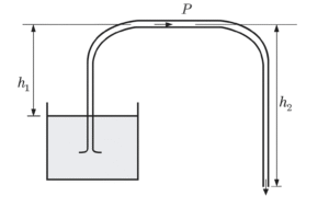
📝 A siphon draws water from a reservoir and discharges it out at atmospheric pressure. Assuming ideal fluid and the reservoir is large, the velocity at point P in the siphon tube is:

(A) $\sqrt{2g h_1}$
(B) $\sqrt{2g h_2}$
(C) $\sqrt{2g(h_2 – h_1)}$
(D) $\sqrt{2g(h_2 + h_1)}$

Solution =

⦾ Given:
✓ Point ①: Surface of the reservoir
✓ Point ②: Exit of the siphon tube (bottom end)
Point P: Top of the siphon (between ① and ②)

Tube has constant diameter, so the velocity is the same at every point
Fluid is ideal (incompressible and no viscosity)

⦾ Step 1: Apply Bernoulli’s Equation between Points ① and ②
\[ \frac{p_1}{\rho g} + \frac{v_1^2}{2g} + z_1 = \frac{p_2}{\rho g} + \frac{v_2^2}{2g} + z_2 \]
Where:
$ p_1 = p_2 = p_{\text{atm}} $ (open to atmosphere)
$ v_1 = 0 $ (surface of large reservoir, so negligible velocity)
$ z_1 = h_2 – h_1 $
$ z_2 = 0 $ (datum line at the siphon outlet)

⦾ Step 2: Substituting into the Bernoulli Equation
\[ \frac{p_{\text{atm}}}{\rho g} + 0 + (h_2 – h_1) = \frac{p_{\text{atm}}}{\rho g} + \frac{v_2^2}{2g} + 0 \]
Cancel $ \frac{p_{\text{atm}}}{\rho g} $ from both sides:
\[ h_2 – h_1 = \frac{v_2^2}{2g} \]
Multiply both sides by $ 2g $:
\[ v_2^2 = 2g(h_2 – h_1) \]
Take square root:
\[ \boxed{v = \sqrt{2g(h_2 – h_1)}} \]

⦾ Conclusion:
Since the siphon tube has constant diameter, the velocity of water is the same throughout the tube. Hence, the velocity at point P is:
\[ \boxed{v_P = \sqrt{2g(h_2 – h_1)}} \]

📝 The head loss for a laminar incompressible flow through a horizontal circular pipe is $ h_1 $. Pipe length and fluid remaining the same, if the average flow velocity doubles and the pipe diameter reduces to half its previous value, the head loss is $ h_2 $. The ratio $ \frac{h_2}{h_1} $ is:

(A) 1
(B) 4
(C) 8
(D) 16

Solution =

The problem involves calculating the ratio of head losses $\frac{h_2}{h_1}$ for laminar flow in a pipe when the velocity and diameter change. The correct answer is C (8).

⦾ Step 1: Hagen-Poiseuille Equation
The head loss $h_f$ for laminar, incompressible flow in a horizontal circular pipe is:
\[ h_f = \frac{32 \mu L \bar{u}}{\rho g D^2} \] ⦾ where:
✓ $\mu$ = dynamic viscosity
✓ $L$ = pipe length
✓ $\bar{u}$ = average flow velocity
✓ $\rho$ = fluid density
✓ $g$ = acceleration due to gravity
✓ $D$ = pipe diameter

⦾ Step 2: Initial Head Loss ($h_1$)
For the initial conditions:
\[ h_1 = \frac{32 \mu L \bar{u}_1}{\rho g D_1^2} \] ⦾ Step 3: New Conditions
The problem states:
Velocity doubles: $\bar{u}_2 = 2\bar{u}_1$
Diameter reduces to half: $D_2 = \frac{D_1}{2}$
The new head loss ($h_2$) becomes:
\[ h_2 = \frac{32 \mu L \bar{u}_2}{\rho g D_2^2} = \frac{32 \mu L (2\bar{u}_1)}{\rho g \left(\frac{D_1}{2}\right)^2} \] ⦾ Step 4: Simplify $h_2$
Simplify the equation step-by-step:
\[ h_2 = \frac{64 \mu L \bar{u}_1}{\rho g \left(\frac{D_1^2}{4}\right)} = \frac{64 \mu L \bar{u}_1 \times 4}{\rho g D_1^2} \] \[ = \frac{256 \mu L \bar{u}_1}{\rho g D_1^2} \] ⦾ Step 5: Compute the Ratio $\frac{h_2}{h_1}$
Divide $h_2$ by $h_1$:
\[ \frac{h_2}{h_1} = \frac{\frac{256 \mu L \bar{u}_1}{\rho g D_1^2}}{\frac{32 \mu L \bar{u}_1}{\rho g D_1^2}} = \frac{256}{32} = 8 \] ⦾ Conclusion: The ratio of head losses is:
\[ \frac{h_2}{h_1} = 8 \] ⦾ Correct Answer: $\boxed{Option C}$

📝 Within a boundary layer for a steady incompressible flow, the Bernoulli equation

(A) holds because the flow is steady
(B) holds because the flow is incompressible
(C) holds because the flow is transitional
(D) does not hold because the flow is frictional

Solution =

The Bernoulli equation is derived under the following assumptions:
✓ Inviscid flow (no friction)
✓ Steady flow
✓ Incompressible flow
✓ Along a streamline

⦾ In the boundary layer:
✓ The flow is viscous (frictional effects are significant).
✓ Shear stresses due to viscosity dominate, causing energy dissipation.
✓ Since the Bernoulli equation neglects viscous effects, it cannot be applied within the boundary layer where friction plays a major role.

⦾ Why the other options are incorrect: (Option => Description => Why Incorrect?)
A => Holds because the flow is steady => Steadiness is necessary but not sufficient (viscosity invalidates Bernoulli)
B => Holds because the flow is incompressible => Incompressibility is required, but viscosity still dominates in the boundary layer
C => Holds because the flow is transitional => Transitional flows are inherently unsteady/viscous, making Bernoulli invalid

⦾ The correct answer is: D) does not hold because the flow is frictional

⦾ Key point: The Bernoulli equation is strictly valid only outside the boundary layer where viscous effects are negligible.

📝 Consider the following statements regarding streamline(s):
(i) It is a continuous line such that the tangent at any point on it shows the velocity vector at that point
(ii) There is no flow across streamlines
(iii) \[ \frac{dx}{u} = \frac{dy}{v} = \frac{dz}{w} \] is the differential equation of a streamline, where $ u, v, w $ are velocities in the directions $ x, y, z $, respectively.
(iv) In an unsteady flow, the path of a particle is a streamline.
Which one of the following combinations of the statements is true?

(A) (i), (ii), (iv)
(B) (ii), (iii), (iv)
(C) (i), (iii), (iv)
(D) (i), (ii), (iii)

Solution =

⦾ Analysis of Statements Regarding Streamlines
(i) It is a continuous line such that the tangent at any point on it shows the velocity vector at that point.
✔️ True — This is the definition of a streamline. The tangent to the streamline represents the direction of the velocity vector at any point.
(ii) There is no flow across streamlines.
✔️ True — Flow is always tangential to streamlines, so there is no component of velocity normal to the streamline.
(iii) \[ \frac{dx}{u} = \frac{dy}{v} = \frac{dz}{w} \] is the differential equation of a streamline, where $ u, v, w $ are velocities in the directions $ x, y, z $, respectively.
✔️ True — This is the correct differential form of streamline equations in 3D.
(iv) In an unsteady flow, the path of a particle is a streamline.
❌ False — In unsteady flow, the path of a particle is a pathline, not a streamline. Streamlines apply only for a fixed instant in time.

⦾ Final Answer:
\[ \text{Correct statements: (i), (ii), (iii)} \]
✔️ Correct Option: D

📝 A flow field which has only convective acceleration is

(A) a steady uniform flow
(B) an unsteady uniform flow
(C) a steady non-uniform flow
(D) an unsteady non-uniform flow

Solution =

⦾ Flow with Only Convective Acceleration
The total acceleration in a fluid flow is given by:
\[ \vec{a} = \frac{\partial \vec{V}}{\partial t} + (\vec{V} \cdot \nabla)\vec{V} \]
$ \frac{\partial \vec{V}}{\partial t} $: Local (temporal) acceleration → present in unsteady flows
$ (\vec{V} \cdot \nabla)\vec{V} $: Convective acceleration → present in non-uniform flows

To have only convective acceleration:
✓ The flow must be steady → no local acceleration
✓ The flow must be non-uniform → convective acceleration is present

⦾ Final Answer:
\[ \boxed{\text{C) a steady non-uniform flow}} \]

📝 Water is coming out from a tap and falls vertically downwards. At the tap opening, the stream diameter is 20 mm with uniform velocity of 2 m/s. Acceleration due to gravity is $9.81 \, \text{m/s}^2 $. Assuming steady, inviscid flow, constant atmospheric pressure everywhere and neglecting curvature and surface tension effects, the diameter in mm of the stream 0.5 m below the tap is approximately

(A) 10
(B) 15
(C) 20
(D) 25

Solution =

⦾ Given:
✓ Initial diameter: $ d_1 = 20 \, \text{mm} = 0.02 \, \text{m} $
✓ Initial velocity: $ v_1 = 2 \, \text{m/s} $
✓ Acceleration due to gravity: $ g = 9.81 \, \text{m/s}^2 $
✓ Height fallen: $ h = 0.5 \, \text{m} $
We are to find the new diameter $ d_2 $ of the stream 0.5 m below the tap.

⦾ Step 1: Find final velocity using energy conservation
\[ v_2^2 = v_1^2 + 2gh \] \[ v_2^2 = 2^2 + 2 \cdot 9.81 \cdot 0.5 = 4 + 9.81 \] \[ = 13.81 \Rightarrow v_2 = \sqrt{13.81} \approx 3.715 \, \text{m/s} \]
⦾ Step 2: Use continuity equation
\[ A_1 v_1 = A_2 v_2 \Rightarrow \frac{\pi d_1^2}{4} \cdot v_1 = \frac{\pi d_2^2}{4} \cdot v_2 \] \[ \Rightarrow d_1^2 \cdot v_1 = d_2^2 \cdot v_2 \Rightarrow d_2 = d_1 \cdot \sqrt{\frac{v_1}{v_2}} \] \[ d_2 = 0.02 \cdot \sqrt{\frac{2}{3.715}} \approx 0.02 \cdot \sqrt{0.538} \] \[ \approx 0.02 \cdot 0.7334 \approx 0.01467 \, \text{m} \] \[ = 14.67 \, \text{mm} \]
⦾ Final Answer:
\[ \boxed{15 \, \text{mm}} \Rightarrow \text{Option B} \]

📝 The maximum velocity of a one-dimensional incompressible fully developed viscous flow, between two fixed parallel plates, is $ 6\, \mathrm{ms}^{-1} $. The mean velocity (in $ \mathrm{ms}^{-1} $) of the flow is

(A) 2
(B) 3
(C) 4
(D) 5

Solution =

In fully developed, one-dimensional, incompressible viscous flow between two parallel plates (also called plane Poiseuille flow), the relationship between maximum velocity and mean velocity is given by:
\[ V_{\text{mean}} = \frac{2}{3} V_{\text{max}} \]
⦾ Given:
\[ V_{\text{max}} = 6\, \text{m/s} \]
Substitute into the formula:
\[ V_{\text{mean}} = \frac{2}{3} \times 6 = 4\, \text{m/s} \]
⦾ Final Answer:
\[ \boxed{\text{C. 4}} \]

📝 In a steady flow through a nozzle, the flow velocity on the nozzle axis is given by $$v = u_0 \left(1 + \frac{3x}{L}\right) i $$ where x is the distance along the axis of the nozzle from its inlet plane and L is the length of the nozzle. The time required for a fluid particle on the axis to travel from the inlet to the exit lane of the nozzle is

(A) $T = \frac{L}{u_0} $
(B) $T = \frac{L}{3u_0} \ln4$
(C) $T = \frac{L}{4u_0} $
(D) $T = \frac{L}{2.5u_0} $

Solution =

The problem asks for the time required for a fluid particle to travel from the inlet ($x=0 $) to the exit ($x=L $) of a nozzle.
The velocity of the fluid particle is given by the equation:
$$v = u_0 \left(1 + \frac{3x}{L}\right)$$ We know that velocity is the rate of change of position with respect to time, so we can write:
$$v = \frac{dx}{dt}$$ Now, we can set up the differential equation:
$$\frac{dx}{dt} = u_0 \left(1 + \frac{3x}{L}\right)$$ To find the time $T $, we need to separate the variables and integrate. Rearranging the equation, we get:
$$dt = \frac{dx}{u_0 \left(1 + \frac{3x}{L}\right)}$$ We need to integrate both sides of the equation. The time goes from $t=0 $ to $t=T $ (the total time we are looking for), and the position goes from $x=0 $ (inlet) to $x=L $ (exit).
$$\int_{0}^{T} dt = \int_{0}^{L} \frac{dx}{u_0 \left(1 + \frac{3x}{L}\right)}$$ First, let’s solve the integral on the left side:
$$\int_{0}^{T} dt = [t]_{0}^{T} = T – 0 = T$$ Now, let’s solve the integral on the right side. We can take the constant $u_0 $ out of the integral:
$$\frac{1}{u_0} \int_{0}^{L} \frac{dx}{1 + \frac{3x}{L}}$$ Let’s use a substitution for the term inside the integral. Let $u = 1 + \frac{3x}{L} $.
To find $du $, we differentiate $u $ with respect to $x $:
$$du = \frac{3}{L} dx \implies dx = \frac{L}{3} du$$ We also need to change the limits of integration.
When $x=0 $, $u = 1 + \frac{3(0)}{L} = 1 $.
When $x=L $, $u = 1 + \frac{3(L)}{L} = 1 + 3 = 4 $.
Now, substitute these into the integral:
$$\frac{1}{u_0} \int_{1}^{4} \frac{1}{u} \left(\frac{L}{3} du\right)$$ Take the constant $\frac{L}{3} $ out of the integral:
$$\frac{L}{3u_0} \int_{1}^{4} \frac{1}{u} du$$ The integral of $\frac{1}{u} $ with respect to $u $ is $\ln|u| $.
$$\frac{L}{3u_0} [\ln|u|]_{1}^{4}$$ Now, apply the limits:
$$\frac{L}{3u_0} (\ln|4| – \ln|1|)$$ Since $\ln(1) = 0 $, the expression simplifies to:
$$\frac{L}{3u_0} (\ln4 – 0) = \frac{L}{3u_0} \ln4$$ So, the total time $T $ is:
$$T = \frac{L}{3u_0} \ln4$$ This matches option B.

📝 For a Newtonian fluid

(A) shear stress is proportional to shear strain
(B) rate of shear stress is proportional to shear strain
(C) shear stress is proportional to rate of shear strain
(D) rate of shear stress is proportional to rate of shear strain

Solution =

For a Newtonian fluid, the relationship between shear stress and the rate of shear strain is given by:
\[ \tau = \mu \frac{du}{dy} \]
⦾ Where:
✓ $ \tau $ = shear stress
✓ $ \mu $ = dynamic viscosity
✓ $ \frac{du}{dy} $ = rate of shear strain (velocity gradient)
This means the shear stress is directly proportional to the rate of shear strain, not to the strain itself.

⦾ Correct Option: C) shear stress is proportional to rate of shear strain.

📝 If x is the distance measured from the leading edge of a flat plate, the laminar boundary layer thickness varies as

(A) $ {1/x} $
(B) $ x^{4/5} $
(C) $ x^{2} $
(D) $ x^{1/2} $

Solution =

For laminar boundary layer flow over a flat plate, the boundary layer thickness $ \delta $ varies with distance $ x $ from the leading edge as per the Blasius solution for steady, incompressible flow:
\[ \delta(x) \propto \sqrt{\frac{\nu x}{U}} \Rightarrow \delta(x) \propto x^{1/2} \]
✓ $ \nu $ is the kinematic viscosity
✓ $ U $ is the free stream velocity
✓ $ x $ is the distance from the leading edge

Therefore, the boundary layer thickness increases as the square root of the distance from the leading edge.

⦾ Correct Answer: D) $ x^{1/2} $

📝 Match the following pairs:

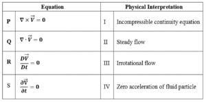
(A) P-IV, Q-I, R-II, S-III
(B) P-IV, Q-III, R-I, S-II
(C) P-III, Q-I, R-IV, S-II
(D) P-III, Q-I, R-II, S-IV

Solution =

⦾ Match the Following Equations to Their Physical Interpretations
P: $ \nabla \times \vec{V} = 0 $
This means the curl of the velocity is zero ⇒ Irrotational flow
✅ P → III
Q: $ \nabla \cdot \vec{V} = 0 $
Divergence of velocity is zero ⇒ Incompressible continuity equation
✅ Q → I
R: $ \frac{D\vec{V}}{Dt} = 0 $
Material derivative is zero ⇒ Zero acceleration of fluid particle
✅ R → IV
S: $ \frac{\partial \vec{V}}{\partial t} = 0 $
Partial derivative with respect to time is zero ⇒ Steady flow
✅ S → II

⦾ Correct Matching:
P → III, Q → I, R → IV, S → II

⦾ Correct Option: C

📝 Froude number is the ratio of

(A) buoyancy forces to viscous forces
(B) inertia forces to viscous forces
(C) buoyancy forces to inertia forces
(D) inertia forces to gravity forces

Solution =

The Froude number (Fr) is a dimensionless number defined as:
\[ Fr = \frac{\text{Inertial force}}{\text{Gravitational force}} = \frac{v}{\sqrt{gL}} \]
⦾ Where:
✓ $ v $ = flow velocity
✓ $ g $ = acceleration due to gravity
✓ $ L $ = characteristic length (e.g., depth of flow)
It is used to compare the influence of inertia to gravity and is especially important in open channel flow, ship hydrodynamics, and wave motion.

⦾ Correct Answer: D) inertia forces to gravity forces

📝 A two-dimensional incompressible frictionless flow field is given by $ \vec{u} = x\hat{x} – y\hat{y} $. If ρ is the density of the fluid, the expression for pressure gradient vector at any point in the flow field is given as

(A) $ \rho(x\hat{x} – y\hat{y}) $
(B) $ -\rho(x\hat{x} + y\hat{y}) $
(C) $ \rho(x\hat{x} + y\hat{y}) $
(D) $ -\rho(x\hat{x} – y\hat{y}) $

Solution =

To determine the pressure gradient vector $\nabla p$ at any point in the given flow field, we will follow these steps:

Given Flow Field:
The velocity field is: \[ \vec{u} = x\hat{x} – y\hat{y} \]
⦾ Step 1: Verify Incompressibility
For a 2D incompressible flow, the divergence of the velocity field must be zero: \[ \nabla \cdot \vec{u} = \frac{\partial u_x}{\partial x} + \frac{\partial u_y}{\partial y} \] \[ = \frac{\partial}{\partial x}(x) + \frac{\partial}{\partial y}(-y) = 1 – 1 = 0 \] The flow is indeed incompressible.

⦾ Step 2: Euler’s Equation (Inviscid Flow)
For a frictionless (inviscid) flow, the Euler equation is: \[ \rho \left( \frac{\partial \vec{u}}{\partial t} + (\vec{u} \cdot \nabla) \vec{u} \right) = -\nabla p + \rho \vec{g} \] Assuming steady flow ($\frac{\partial \vec{u}}{\partial t} = 0$) and neglecting body forces ($\vec{g} = 0$), the equation simplifies to: \[ \rho (\vec{u} \cdot \nabla) \vec{u} = -\nabla p \]
⦾ Step 3: Compute the Convective Acceleration $(\vec{u} \cdot \nabla) \vec{u}$
First, compute $\vec{u} \cdot \nabla$: \[ \vec{u} \cdot \nabla = u_x \frac{\partial}{\partial x} + u_y \frac{\partial}{\partial y} = x \frac{\partial}{\partial x} – y \frac{\partial}{\partial y} \]
Now apply this operator to $\vec{u}$: \[ (\vec{u} \cdot \nabla) \vec{u} = \left( x \frac{\partial}{\partial x} – y \frac{\partial}{\partial y} \right) (x\hat{x} – y\hat{y}) \] \[ = x \frac{\partial}{\partial x}(x\hat{x} – y\hat{y}) – y \frac{\partial}{\partial y}(x\hat{x} – y\hat{y}) \] \[= x \left( \frac{\partial x}{\partial x}\hat{x} – \frac{\partial y}{\partial x}\hat{y} \right) – y \left( \frac{\partial x}{\partial y}\hat{x} – \frac{\partial y}{\partial y}\hat{y} \right) \] \[ = x (1\hat{x} – 0\hat{y}) – y (0\hat{x} – 1\hat{y}) \] \[ = x\hat{x} + y\hat{y} \]
⦾ Step 4: Relate to Pressure Gradient
From Euler’s equation: \[ \rho (\vec{u} \cdot \nabla) \vec{u} = -\nabla p \] Substitute the convective acceleration: \[ \rho (x\hat{x} + y\hat{y}) = -\nabla p \] Solve for $\nabla p$: \[ \nabla p = -\rho (x\hat{x} + y\hat{y}) \]
⦾ Final Answer: The expression for the pressure gradient vector is: \[ -\rho(x\hat{x} + y\hat{y}) \]
⦾ Correct Option: B \[ -\rho(x\hat{x} + y\hat{y}) \]

📝 Kaplan water turbine is commonly used when the flow through its runner is

(A) axial and the head available is more than 100 m.
(B) axial and the head available is less than 10 m.
(C) radial and the head available is more than 100 m.
(D) mixed and the head available is about 50 m.

Solution =

⦾ Kaplan Turbine:
✓ Type: Axial flow reaction turbine
✓ Head range: Low head, typically less than 30 meters
✓ Flow: Axial flow through the runner
✓ Application: High flow rate, low head hydropower plants

⦾ Now examine the options:
A. Axial and the head available is more than 100 m
❌ Incorrect — Head is too high for Kaplan turbine.
B. Axial and the head available is less than 10 m
✅ Correct — Kaplan is designed for low head and axial flow.
C. Radial and the head available is more than 100 m
❌ Incorrect — Kaplan is axial, not radial.
D. Mixed and the head available is about 50 m
❌ Incorrect — This applies more to Francis turbine, not Kaplan.

⦾ Final Answer: B) Axial and the head available is less than 10 m

📝 For an incompressible flow field $ \vec{V} $, which one of the following conditions must be satisfied?

(A) $ \nabla \cdot \vec{V} = 0 $
(B) $ \nabla \times \vec{V} = 0 $
(C) $ (\vec{V} \cdot \nabla) \vec{V} = 0 $
(D) $ \frac{\partial \vec{V}}{\partial t} + (\vec{V} \cdot \nabla) \vec{V} = 0 $

Solution =

The condition for incompressible flow is that the divergence of the velocity field is zero:
\[ \nabla \cdot \vec{V} = 0 \]
This ensures the fluid density is constant and there’s no net volumetric expansion or compression.

📝 In order to have maximum power from a Pelton turbine, the bucket speed must be

(A) equal to the jet speed
(B) equal to half of the jet speed.
(C) equal to twice the jet speed.
(D) independent of the jet speed.

Solution =

In a Pelton turbine, water jets hit the buckets and transfer kinetic energy.
Maximum efficiency (and hence maximum power) occurs when the relative velocity of water with respect to the moving bucket results in zero velocity at exit, minimizing energy loss.
From impulse turbine theory, this condition is satisfied when: \[ u = \frac{V}{2} \] ⦾ where:
✓ $ u $ = bucket speed
✓ $ V $ = jet speed
Therefore, the correct choice is:
\[ \boxed{\text{B. equal to half of the jet speed}} \]

📝 Consider steady, incompressible and irrotational flow through a reducer in a horizontal pipe where the diameter is reduced from 20cm to 10cm. The pressure in the 20cm pipe just upstream of the reducer is 150 kPa. The fluid has a vapor pressure of 50kPa and a specific weight of $ 5 \, \text{kN/m}^3 $ Neglecting frictional effects, the maximum discharge that can pass through the reducer without causing cavitation is $ \text{m}^3/\text{s}$

(A) 0.05
(B) 0.16
(C) 0.27
(D) 0.38

Solution =

⦾ Given:
✓ Diameter changes from $ D_1 = 0.2 \, \text{m} $ to $ D_2 = 0.1 \, \text{m} $
✓ Pressure at section 1: $ P_1 = 150 \, \text{kPa} $
✓ Vapour pressure at section 2: $ P_v = 50 \, \text{kPa} $
✓ Specific weight: $ \gamma = 5 \, \text{kN/m}^3 = 5000 \, \text{N/m}^3 $

⦾ Step 1: Apply Bernoulli’s equation (horizontal pipe, so elevation cancels)
\[ \frac{P_1}{\gamma} + \frac{v_1^2}{2g} = \frac{P_2}{\gamma} + \frac{v_2^2}{2g} \]
Set $ P_2 = P_v $ (to avoid cavitation).

⦾ Step 2: Calculate cross-sectional areas
\[ A_1 = \frac{\pi}{4} D_1^2 = \frac{\pi}{4} (0.2)^2 = 0.0314 \, \text{m}^2 \] \[ A_2 = \frac{\pi}{4} D_2^2 = \frac{\pi}{4} (0.1)^2 = 0.00785 \, \text{m}^2 \]
⦾ Step 3: Express velocities in terms of discharge $ Q $
\[ v_1 = \frac{Q}{A_1}, \quad v_2 = \frac{Q}{A_2} \]
⦾ Step 4: Substitute into Bernoulli’s equation
\[ \frac{150000}{5000} + \frac{1}{2g} \left( \frac{Q}{0.0314} \right)^2 \] \[ = \frac{50000}{5000} + \frac{1}{2g} \left( \frac{Q}{0.00785} \right)^2 \]
⦾ Step 5: Simplify
\[ 30 + \frac{1}{2g} \left( \frac{Q^2}{0.0314^2} \right) \] \[ = 10 + \frac{1}{2g} \left( \frac{Q^2}{0.00785^2} \right) \]
Multiply through by $ 2g $:
\[ 60g + \frac{Q^2}{0.0314^2} = 20g + \frac{Q^2}{0.00785^2} \]
\[ 40g = Q^2 \left( \frac{1}{0.00785^2} – \frac{1}{0.0314^2} \right) \]
⦾ Step 6: Compute values
\[ \frac{1}{0.00785^2} \approx 16233, \quad \frac{1}{0.0314^2} \approx 1014 \] \[ \Rightarrow \text{Difference} = 15219 \]
⦾ Step 7: Solve for $ Q $
\[ 40 \times 9.81 = Q^2 \times 15219 \] \[ \Rightarrow Q^2 = \frac{392.4}{15219} \Rightarrow Q^2 \approx 0.02578 \] \[ \Rightarrow Q \approx 0.1605 \, \text{m}^3/\text{s} \]
⦾ Final Answer: $\boxed{0.16 \, \text{m}^3/\text{s}}$

⦾ Correct option: B

📝 Consider an incompressible laminar boundary layer flow over a flat plate of length L, aligned with the direction of an oncoming uniform free stream. If F is the ratio of the drag force on the front half of the plate to the drag force on the rear half, then

(A) $ F < \frac{1}{2} $
(B) $ F = \frac{1}{2} $
(C) $ F = 1 $
(D) $ F > 1 $

Solution =

Consider an incompressible laminar boundary layer flow over a flat plate of length $ L $, aligned with the direction of an oncoming uniform free stream. Let
$ F = \frac{\text{Drag on front half}}{\text{Drag on rear half}} $

⦾ Drag Force for Laminar Flow on a Flat Plate:
The local shear stress is proportional to:
\[ \tau(x) \propto \frac{1}{\sqrt{x}} \]
So the drag force is the integral of shear stress:
\[ \text{Drag} \propto \int \tau(x) \, dx \propto \int \frac{1}{\sqrt{x}} \, dx \]
✓ Front half: $ x = 0 $ to $ x = \frac{L}{2} $
\[ F_1 \propto \int_0^{L/2} \frac{1}{\sqrt{x}} dx = 2\sqrt{x} \Big|_0^{L/2} \] \[ = 2\sqrt{\frac{L}{2}} = \sqrt{2L} \]
✓ Rear half: $ x = \frac{L}{2} $ to $ x = L $
\[ F_2 \propto \int_{L/2}^{L} \frac{1}{\sqrt{x}} dx = 2\sqrt{x} \Big|_{L/2}^{L} \] \[ = 2\left( \sqrt{L} – \sqrt{\frac{L}{2}} \right) \]
Now, the ratio $ F $:
\[ F = \frac{F_1}{F_2} = \frac{\sqrt{2L}}{2\left( \sqrt{L} – \sqrt{\frac{L}{2}} \right)} \] \[ = \frac{\sqrt{2}}{2\left(1 – \frac{1}{\sqrt{2}} \right)} \]
\[ = \frac{\sqrt{2}}{2 \cdot \frac{\sqrt{2} – 1}{\sqrt{2}}} = \frac{\sqrt{2} \cdot \sqrt{2}}{2(\sqrt{2} – 1)} \] \[ = \frac{2}{2(\sqrt{2} – 1)} = \frac{1}{\sqrt{2} – 1} \]
Now rationalize the denominator:
\[ F = \frac{1}{\sqrt{2} – 1} \cdot \frac{\sqrt{2} + 1}{\sqrt{2} + 1} = \frac{\sqrt{2} + 1}{1} \] \[ = \sqrt{2} + 1 \approx 1.414 + 1 = 2.414 \]

⦾ Final Answer:
\[ \boxed{D. \quad F > 1} \]

📝 A venturimeter of 20 mm throat diameter is used to measure the velocity of water in a horizontal pipe of 40 mm diameter. If the pressure difference between the pipe and throat sections is found to be 30 kPa then, neglecting frictional losses, the flow velocity is

(A) 0.2 m/s
(B) 1.0 m/s
(C) 1.4 m/s
(D) 2.0 m/s

Solution =

⦾ Given:
✓ Throat diameter ($d_2$): 20 mm = 0.02 m
✓ Pipe diameter ($d_1$): 40 mm = 0.04 m
✓ Pressure difference ($P_1 – P_2$): 30 kPa = 30,000 Pa
✓ Density of water ($\rho$): 1000 kg/m³
Neglect frictional losses.

⦾ Steps:
1. Find the Area Ratio
The cross-sectional areas of the pipe ($A_1$) and throat ($A_2$) are: \[ A_1 = \frac{\pi d_1^2}{4} = \frac{\pi (0.04)^2}{4} \] \[ = 1.2566 \times 10^{-3} \, \text{m}^2 \] \[ A_2 = \frac{\pi d_2^2}{4} = \frac{\pi (0.02)^2}{4} \] \[ = 3.1416 \times 10^{-4} \, \text{m}^2 \]
The area ratio is: \[ \frac{A_1}{A_2} = \left( \frac{d_1}{d_2} \right)^2 = \left( \frac{40}{20} \right)^2 = 4 \]
2. Apply Bernoulli’s Equation and Continuity Equation
For a venturimeter, neglecting losses, Bernoulli’s equation between the pipe (section 1) and throat (section 2) is: \[ P_1 + \frac{1}{2} \rho v_1^2 = P_2 + \frac{1}{2} \rho v_2^2 \] Rearranging: \[ P_1 – P_2 = \frac{1}{2} \rho (v_2^2 – v_1^2) \]
From the continuity equation (assuming incompressible flow): \[ A_1 v_1 = A_2 v_2 \] \[ \implies v_2 = \left( \frac{A_1}{A_2} \right) v_1 = 4 v_1 \]
Substitute $ v_2 = 4 v_1 $ into the pressure difference equation: \[ P_1 – P_2 = \frac{1}{2} \rho \left( (4 v_1)^2 – v_1^2 \right) \] \[ 30,000 = \frac{1}{2} \times 1000 \times (16 v_1^2 – v_1^2) \] \[ 30,000 = 500 \times 15 v_1^2 \] \[ 30,000 = 7500 v_1^2 \] \[ v_1^2 = \frac{30,000}{7500} = 4 \] \[ v_1 = \sqrt{4} = 2 \, \text{m/s} \]

⦾ Answer: The flow velocity in the pipe is 2.0 m/s.

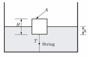
📝 A cylindrical body of cross -sectional area A, height H and density $ \rho_s $, is immersed to depth h in a liquid of density $ \rho $, and tied to the bottom with a string .The tension in the string is

(A) $ \rho g h A $
(B) $ (\rho_s – \rho) g h A $
(C) $ (\rho – \rho_s) g h A $
(D) $ (\rho h – \rho_s H) g A $

Solution =

⦾ Given:
✓ Cross-sectional area of the cylinder = $ A $
✓ Height of the cylinder = $ H $
✓ Density of the solid (cylinder) = $ \rho_s $
✓ Immersed depth = $ h $
✓ Density of the liquid = $ \rho $
✓ Acceleration due to gravity = $ g $
✓ Tension in the string = $ T $ (to be determined)

⦾ Step 1: Weight of the cylinder
\[ W = \text{Volume} \times \text{Density} \times g \] \[ = (A \cdot H) \cdot \rho_s \cdot g = \rho_s g H A \]
⦾ Step 2: Buoyant Force (Upward)
\[ F_B = \text{Submerged Volume} \] \[ \times \text{Liquid Density} \times g \] \[ = (A \cdot h) \cdot \rho \cdot g = \rho g h A \]
⦾ Step 3: Apply Equilibrium Condition
The cylinder is at rest and tied down, so the net force is zero. Taking upward as positive:
\[ \text{Buoyant Force} – \text{Weight} – T = 0 \] \[ \rho g h A – \rho_s g H A – T = 0 \] \[ T = \rho g h A – \rho_s g H A \] \[ \boxed{T = (\rho h – \rho_s H) g A} \]

📝 A horizontal shaft centrifugal pump lifts water at 65 C. The suction nozzle is one meter below pump centerline. The pressure at this point equal 200 kPa gauge and velocity is 3 m/s. Steam tables show saturation pressure at 65 C is 25 kPa, and specific volume of the saturated liquid is $ v = 0.001020 \, \text{m}^3/\text{kg} $. The pump Net Positive suction Head (NPSH) in meters is:

(A) 24
(B) 26
(C) 28
(D) 30

Solution =

⦾ Given:
✓ Temperature of water: $ T = 65^\circ C $
✓ Suction height below pump centerline: $ h_s = 1 \, \text{m} $
✓ Gauge pressure at nozzle inlet: $ p_{1,g} = 200 \, \text{kPa} $
✓ Atmospheric pressure: $ p_{\text{atm}} = 101.325 \, \text{kPa} $
✓ Velocity at suction nozzle: $ V_s = 3 \, \text{m/s} $
✓ Saturation (vapor) pressure at 65°C: $ p_v = 25 \, \text{kPa} $
✓ Specific volume: $ v = 0.001020 \, \text{m}^3/\text{kg} $
✓ Gravitational acceleration: $ g = 9.81 \, \text{m/s}^2 $

⦾ Convert Gauge Pressure to Absolute Pressure:
\[ p_{1,\text{abs}} = p_{1,g} + p_{\text{atm}} = 200 + 101.325 \] \[ = 301.325 \, \text{kPa} = 301.325 \times 10^3 \, \text{Pa} \]
Calculate Density:
\[ \rho = \frac{1}{v} = \frac{1}{0.001020} = 980.39 \, \text{kg/m}^3 \]
Apply Bernoulli’s Equation to Calculate NPSH:
\[ \text{NPSH} = \frac{p_{1,\text{abs}}}{\rho g} + \frac{V_s^2}{2g} – h_s – \frac{p_v}{\rho g} \]
Substituting Values:
⦾ Step 1: $ \frac{p_{1,\text{abs}}}{\rho g} $
\[ \frac{301325}{980.39 \times 9.81} = \frac{301325}{9612.63} \approx 31.33 \, \text{m} \]
⦾ Step 2: $ \frac{V_s^2}{2g} $
\[ \frac{3^2}{2 \cdot 9.81} = \frac{9}{19.62} \approx 0.458 \, \text{m} \]
⦾ Step 3: Suction height
\[ -h_s = -1 \, \text{m} \]
⦾ Step 4: $ \frac{p_v}{\rho g} $
\[ \frac{25000}{980.39 \times 9.81} = \frac{25000}{9612.63} \approx 2.60 \, \text{m} \]
⦾ Final NPSH:
\[ \text{NPSH} = 31.33 + 0.458 – 1 – 2.60 \] \[ = 28.188 \approx \boxed{28 \, \text{m}} \]
⦾ Correct Answer: Option C) 28

Upgrade to Premium & get extra PYQs

250+

Go Premium

GATECAREER

Fluid Mechanics PYQ Set (2000 to 2025)

Upgrade to Premium & get extra PYQs

Engineering Calculator